-
The emperor’s new clothes

This is one of the most insightful fairy tales. The most famous rendition is by Hans Christian Andersen, but, according to Wikipedia, there are various earlier versions around. Here is a very short version. Swindlers sell the king what they claim to be a magnificent set of new clothes with the feature that only competent or clever people can see them. When a series of officials and then the king himself inspect the new clothes, they see nothing but pretend otherwise. Eventually, the king leads a procession through the town and still everyone claims to see the magnificent clothes until a child finally cries out that the emperor is naked. At this point, everyone realizes that they have been fooled. In this blog post, I want to provide a first decision-theoretic and then game-theoretic underpinning for this story (with a big thank you to PB). I will use psychological game theory, even if that’s not strictly necessary, and one can also see it a bit as rational herding.
Let me first look at this problem from just one person’s point of view. This person should probably realize that there are two possibilities: that what the swindlers say is true or that this is all a hoax. The swindlers probably didn’t introduce themselves as swindlers, only we the reader already know that there are swindlers. But a reasonable person should arguably attach at least some positive probability to the possibility that this is a hoax, in which case even clever people would see no clothes. Call this (subjective) probability of a hoax
some number between zero and one, with
the (subjective) probability of the swindlers being truthful. Next, let me allow for the possibility that this person we are looking at does not fully know whether or not they are stupid. Let
also between zero and one, be this (subjective) probability of being stupid, with
the (subjective) probability of being not stupid, call it clever. Suppose that this person, furthermore, if they believe the swindlers to be truthful, believes that they are fully truthful. This means that there are only stupid and clever people (nothing in between) and stupid people, with probability one, do not see the clothes, while clever people see the clothes with probability one. If the whole thing is a hoax, then, of course, everyone, clever or stupid, would see no clothes.
Now suppose, as seems to be the relevant case at hand, that this person doesn’t see any clothes. If this person is rational, despite perhaps being stupid, what should this person now believe about their own stupidity and about whether or not the whole affair is a hoax? We are interested in the probability that this person is stupid conditional on this person seeing no clothes, which is given by
Why? The numerator is equal to
because the probability of being stupid and seeing no clothes is the same as that of being stupid. After all, irrespective of whether this is a hoax or true, a stupid person would not see any clothes. The denominator is equal to
because in the case of the whole thing being a hoax, probability
only stupid people, probability
Anyway, what does this mean? Well, it means that this person when seeing no clothes updates their belief about their own stupidity to something higher than before, as long as
(otherwise they are ex-ante sure that this is a hoax, in which case they learn nothing about their own stupidity from seeing no clothes) and as long as
(otherwise they know they are clever and no evidence can change that). Perhaps importantly, if this person is fairly sure that the whole thing is no hoax, that is when
is close to zero, then the fact that they see no clothes would essentially tell them with almost certainty that they are stupid.
We can similarly compute this person’s updated belief about the whole affair being a hoax. The probability of that is given by
This person will, therefore, also think that the probability that this is a hoax has gone up after they see no clothes provided
(otherwise they are sure that this is all true, and no amount of evidence can change that) and provided
(otherwise they are sure they are stupid and so they learn nothing about whether or not this is a hoax from seeing no clothes).
So, this is what this rational, yet possibly stupid, person learns from the fact that they see no clothes. But why do they not honestly declare that they have not seen any clothes? To answer that properly, we need to think about the other people involved in this interaction and this takes us to game theory.
The, or at least a way to rationalize this person’s behavior is by assuming that they care about what others think of them. Their utility from their own (and everybody else’s) actions depends (at least to a sufficient extent) on the induced posterior beliefs that the other people have about this person’s stupidity that arise from these actions. If this is what we assume, we are in fact in the more recently developed realm of psychological game theory (See this 2022 article by Battigalli and Dufwenberg for a recent survey). In standard game theory, utilities (also called payoffs) only depend on states and actions, not on beliefs. Having said that, there is an easy, and not entirely implausible, way to use standard game theory here as well. Instead of caring about what others think of them, people (especially those officials perhaps) might just care about keeping their job, and they keep their job only if they are deemed clever. But I do think that psychological game theory is, if nothing else, at least a nice shortcut to modeling situations such as this one.
Anyway, let us assume that everybody involved in this interaction cares mostly about what others think of them: the subjective probability that others attach to them being stupid negatively enters the utility function. For instance, a concrete model could have a utility function for a person of minus the average subjective probability that others attach to this person being stupid.
When you think about it this way, you realize that how certain a person is about their own stupidity is not so very relevant to their own choices. Even if you know that you are clever, and, therefore, when seeing no clothes, know that this is all a hoax, you might say that you see clothes. It all depends on whether the others know that you are clever. If others are unsure whether you are clever or not, then you will say you see clothes so that the others don’t think that you are stupid, even if you know that you are not.
So, when you see no clothes, and are asked to make a public statement about what you saw, the relevant parameters are not your own assessments
This is also why it is not enough for one person (who privately thinks themselves very clever) to declare that they have seen no clothes for all to suddenly realize that this is a hoax. For this to happen, it takes a person, who everybody sees as not possibly being stupid, to declare that the emperor is naked. I am not sure why a child satisfies this criterion, but I seem to remember that there was an argument in the story – maybe it was not about stupidity, but about being an adulterer or -ess, or something else that could not possibly apply to a child, but could apply to all adults.
I now want to finally turn to the social dilemma that this behavior induces. In the story, there is a series of people who observe the state of the king’s clothing and they successively (somewhat publicly) declare that they see clothes. So far, I have, essentially, only argued why the first person might declare that they see clothes when they do not. But if the second person understands that the first person would always declare to have seen clothes, irrespective of what they have actually seen – and a bit of introspection might lead to this conclusion – they have learned nothing from the first person’s statement. So, the problem for the second person is just the same as that for the first person. As long as nobody has declared to have seen no clothes, the problem is the same for everyone (ok, this is true under the assumption that we are all somewhat alike). The tragedy of this phenomenon is that, if it hadn’t been for the child, nobody would have learned that the swindlers were exactly that, swindlers. Everybody would have privately updated the chance of this being a hoax to a slightly higher probability, yet all together they would have had enough information to find out the truth. If everybody (against their incentives) had truthfully declared what they saw, all would have quickly found out that nobody had seen any clothes, and as long as they all believe that there is at least some proportion of non-stupid people in this town (that is that
), they would have realized that the chance of this being a hoax, conditional on all this information, is pretty close to one. The behavior of the people in the story of the emperor’s new clothes, thus, prevents learning, somewhat like in the case of rational herding (as in a previous post) where learning stops after people start to discard their own information and imitate others instead.
-
The equilibrium exam

If there is one thing that I don’t enjoy about working at a university, it is grading. There are two aspects of grading that I don’t enjoy. One is simply the pure “manual” labor (I guess it isn’t quite manual – but it sure feels like it) that goes into reading the exam papers and trying to decipher what is written and trying to match the appropriate number of points to the partially correct answers in a consistent manner. Some of my colleagues do this while listening to military marches by the Johann Strausses, for instance, for better endurance results. But this is the less interesting aspect. The second is the more general job of assigning grades to people. I would much prefer to just teach them some interesting stuff without having to test them, but I understand that, even if I don’t like it, they would learn less of what I try to teach them if I didn’t test and grade them. Also, as examiners, it is part of our job to provide valuable information for the potential employers of our students (the signaling value of receiving an education). And testing is interesting as it is a bit of a game between me, who chooses what to test, and the students, who choose how much and what (if any) to study for the exam.
There are many interesting game-theoretic aspects of testing students. For instance, for me as an examiner, should or should I not use old exam questions? Ideally, I convince the students that they will certainly get new ones, and then actually use some old ones. And, as I typically cannot test everything I have done in a course, which topics should I test? Game theory would probably tell me that I should randomize (in both of these problems), which is in fact what I do, to some extent. The students, on the other hand, have the problem of how much and what to study. Do they study all the material or should they gamble on me not testing some of the topics and only study a subset of the material? How deeply do they need to understand stuff? Is it enough if they can repeat all definitions without fully understanding them or should they at least learn some of the recipes to solve certain problems or do they even need to really understand what has been taught? I certainly would like them to study so that they understand it all deeply, but I am not sure I always succeed. Well, I am, in fact, sure that I don’t always succeed. Well well, I don’t want to say it, but I probably actually never succeed.
But let me talk about another problem that I have, the problem of how hard the exam should be. I have two goals when I am teaching: One, I want the students to learn and comprehend interesting and useful new things; two, I would ideally like them to have good grades. [We don’t use a fixed grade distribution.] And what I noticed is this: the easier I make the exam the more the grade distribution doesn’t change. Ok, this is both grammatically and empirically not completely correct. When I make the exam easier, grades do go up a bit (they are on average better) with two caveats. One, this is more true for an exam that I just made easier relative to previous ones, but then grades go down a bit in the next exam with the same degree of difficulty. Second, this effect is less pronounced than I would have hoped. In fact, I have the feeling that there is no (low) degree of difficulty that I could choose that would induce all students to pass the course.
And why is this? Well, this is so because students choose their level of study effort strategically. I believe this to be true even for some of my students who are skeptical about what I teach them about people responding to incentives. If students expect the exam to be easy, they don’t study very hard. If they expect the exam to be hard, they also study hard, or at least harder. And this effect makes it hard for me to consistently create exams that induce students to get good grades. I guess, I should probably learn from this and care less about the grades and more about what the students learn. So, the next exams will be harder! I hope my students are reading this.
-
The helmet and safety jacket dilemma

When my children bike to school, they wear a helmet. When they use a (non-electric) scooter, they don’t. They also don’t wear any bright and highly visible safety jackets when using either. Why not? I certainly would prefer if they did and I tell them so. But they don’t want to. They have a variety of arguments, the jacket doesn’t fit properly, they can’t see well with the helmet, et cetera. But I suspect that the real reason is that it is not considered cool to wear a helmet on a scooter or a safety jacket on either scooter or bike. I speak of children, but I have the feeling that adults are not so different. Nobody used to use seatbelts (although why that may have been considered cool, I don’t know) and nobody wore a helmet on motorbikes and now, when everybody has to, nobody seems to mind. Not many adults wear helmets when they are biking and, at least in Graz where I live, not many use helmets even on those e-bikes, some of which look like and are almost as fast as motorbikes. In this post, I want to provide a simple game theoretic model that allows me to study how wanting to be cool could influence people’s decisions when it comes to helmets and such things and to see how much of a social dilemma this might induce.
I will model this problem as a population game. There is a continuum (a large number) of (each on their own non-influential) people. Each person decides to wear a helmet or not (when biking or scooting or whatever it is). When making this decision they care about the proportion of others that wear a helmet. I will allow people to have somewhat different preferences from each other, not everybody feels the same way about wearing helmets. The model can be summarized by two ingredients, a personal characteristic
that is distributed in the population according to some cumulative distribution function
, and a utility function
, a person’s utility when wearing a helmet, that depends on the proportion
of people that wear helmets and on their characteristic
For simplicity, I will choose a specific, slightly crude, functional form for this utility function:
where the
is the (obviously assumed positive) net benefit from wearing a helmet (increased chance of survival minus any discomfort that wearing a helmet might induce) and
is the feeling of shame when wearing a helmet for all to see. This latter expression is chosen to have a few key features. First, the higher
(I am breaking indifference in favor of wearing helmets, but this is not important). By design, this means that a person will wear a helmet if and only if
. In other words,
will always wear a helmet, regardless of how many others wear helmets, and that a person with a
will never wear a helmet.
In this world that I just created, there is a best and worst possible outcome. The fewer people wear helmets the (weakly) worse off everyone is: either they don’t wear a helmet anyway, then they are unaffected, or they wear a helmet when many people do, but not when only a few do, in which case their utility has gone down, or they wear a helmet in either case, then their feeling of shame for wearing one has gone up. The best outcome is the one, in which everyone (other than a type
The worst outcome is the one, in which nobody (other than types
, for types
We are now looking for (Nash) equilibria of this game. An equilibrium proportion
is given by the cumulative distribution function
In equilibrium, we, thus, simply must have that
Suppose we assume, as seems reasonable, that there are people who will always wear a helmet regardless of how many others wear a helmet, and that there are people who will never voluntarily wear a helmet. This means that
and
Given that
So, we must have at least one equilibrium. What equilibrium we can get all depends on
the distribution of
that is, the distribution of people’s attitude towards the societal shame they feel when wearing a helmet.
To discuss some of the many different possible situations I use a series of high-tech pictures with the proportion of people wearing a helmet
and the cumulative distribution function
.

In the situation that I denoted “lucky,” there are many people with a low
In this case, there is a unique equilibrium and it has a high proportion of people wearing helmets. By the way, if you are wondering how we would get to this equilibrium, there is a dynamic or evolutionary justification. Suppose nobody is wearing a helmet and helmets have just been introduced. Then
is the proportion of people who immediately take up helmets. Call this
Others now realize that there are a proportion of
people wearing helmets. This induces others to take up helmets. It would induce about
new people to take up helmets. We then have a proportion of
of people wearing helmets. This goes on and on, until we hit the equilibrium point where
And when we get there, this would be all great.
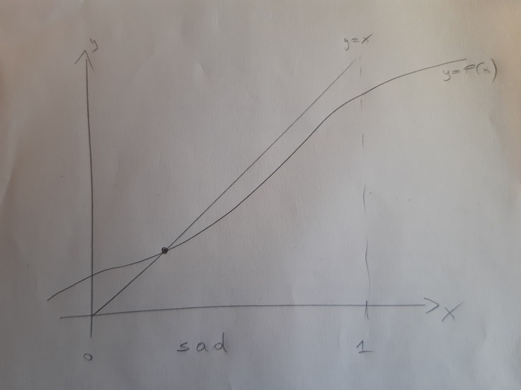
In contrast, in the picture that I titled “sad”, most people are very worried about societal shame. This can be seen in the slow rise of
in
How could we get from the latter situation to the former? There are, actually, many ways a government could try to make that happen. One option would be to make helmets mandatory (and to enforce this rule at least to some extent) so that, presumably, people suffer a cost for not wearing a helmet, the fine they might receive when caught, which makes wearing a helmet relatively more attractive for them. This could be expensive, as you need to hire and pay police personnel to enforce the rules. Another option that the government could try to use is to fund an advertising campaign aimed at making people less worried about not being cool. They could try to make wearing helmets cool, instead, for instance. This could have just the same effect. Under both policy measures, if done well, the function
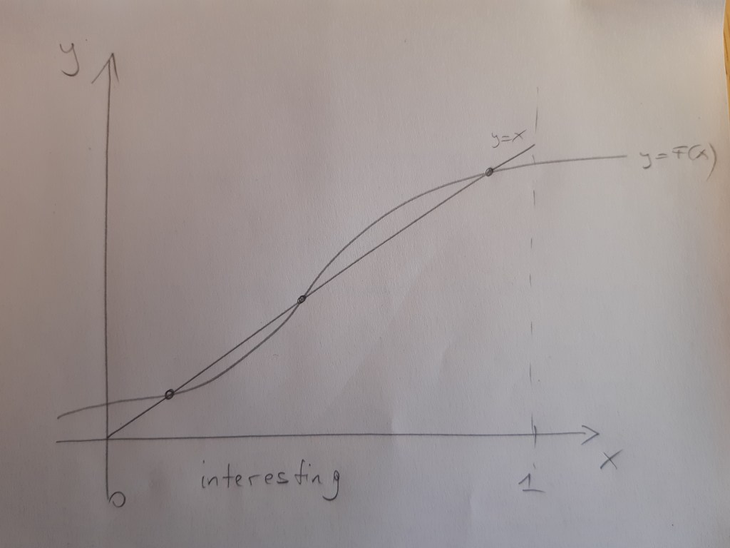
There is a third possible situation, that I depict in the figure entitled “interesting,” in which there are multiple equilibria. The low and high helmet-wearing equilibria are both dynamically stable (a dynamic process as the one I described above would lead to these points when the system starts in the vicinity of these points). The middle equilibrium is not dynamically stable. The lower equilibrium is initially more likely, as it makes sense to think that at some initial point, nobody wore helmets. If this is the situation that we are facing, then introducing a law to make helmets mandatory needs to be implemented and enforced only for a short time, until the proportion of helmet wearers exceeds the middle (unstable) equilibrium. After that we end up in the good equilibrium without any need for further enforcement.
This post has become a bit longer than I intended. Of course, one could debate whether or not there really is a social dilemma here (meaning my utility functions are possibly wrong). Perhaps, people just value the freedom of having the wind blow through their hair when scooting much more than the added chance of survival from a possible accident. Then a helmet law would make everybody just worse off. An advertising campaign might not be so bad in that case. There are many other things one could question, but I won’t do this now.
-
Rational Herding on the Autobahn

The speed limit on the Autobahn south of Graz to the Austrian/Slovenian border varies. Sometimes the speed limit is 130 km/h and sometimes it is 100 km/h. The speed limit is also not constant for the whole stretch of Autobahn and, after some distance from Graz, it definitely becomes 130 km/h. I don’t fully understand how these speed limit decisions are made and I also don’t quite know at which point the speed limit is definitely 130 km/h. I believe it has something to do with local pollution, so it may depend on weather or traffic conditions, but I don’t quite know. So, at least for me, the speed limit is a random variable and this is probably also true for most people. Now, what should I do when I am somewhere on this Autobahn at a point, where I am not sure what the speed limit is? I rationally “herd”.
Let me explain. To inform people about the speed limit, there are some, not many, electronic signs that can be programmed from some central place. The other day, when I drove south from Graz, I was initially in no doubt about the speed limit. One of these electronic signs just outside Graz was clearly showing 100 km/h. So, I attached a probability pretty close to 1 to the event (as probability theorists like to call it) that the speed limit is 100 km/h and I drove accordingly. A little bit later there was another one of these signs and that sign, if anything, just made my subjective probability assessment of the event that the speed limit is 100 km/h even closer to 1, and I still drove accordingly. I then drove on for quite some time, perhaps 10 or 20 kilometers, a little bit lost in thought, when I realized that I hadn’t seen a speed limit sign recently. Did I miss them? There should have been one, I thought, and I probably didn’t notice it. So, what was the speed limit now?
I also noticed, and that possibly prompted my reevaluation of my speed limit beliefs, that I was being overtaken by some cars that were going pretty fast. You need to know that drivers on the Austrian Autobahn, by and large, obey the speed limits. Of course, this is not 100% true, and one has to take this into consideration. But with any car that I estimated to be going about 130km/h when they overtook me, my subjective probability assessment that the speed limit is 100km/h went down and down and down. After about 4 or 5 cars went past me at about 130 km/h, I was at the point where I attached a sufficiently high probability to the event that the speed limit is 130km/h that I also went 130 km/h. I didn’t need this probability to be 1, as the chances of being caught speeding and being fined for it are not that high, and I, of course, preferred to get to wherever I wanted to get to earlier rather than later.
After a few minutes of driving speedily along, I encountered the next speed sign and it showed 100 km/h. There is a small probability that the speed limit had been temporarily (I mean on that stretch of Autobahn that I just had been on) 130 km/h, but it is a small one. So, I and the other drivers were wrong. Or were we? I would like to say that I was not wrong because I did not attach a probability of 1 to the event that the speed limit was 130 km/h. And possibly the other drivers also did not. The question is this: did or did we not also take into account that some of the other drivers that were going 130 km/h were going 130 km/h because they had seen others go 130 km/h and had formed their belief on a similar basis as I did. It is quite possible (and perhaps we did take this into account) that the first driver that we all saw going 130 km/h did this by mistake or just because they didn’t care. Perhaps this one driver was already enough, however, for a second driver to change their beliefs sufficiently for them to increase their speed and that, in turn, prompted a third and that a fourth and that me to start to go faster.
All of these decisions could be declared as being rational decisions as long as none of us were fooled into believing with certainty that the speed limit was now 130 km/h. We imitated the behavior of others before us, rationally thinking that their behavior provided evidence that the speed limit was 130 km/h. Often this assessment would have been correct. In the present case, it was not. This is, unfortunately, something that can happen when people rationally “herd on” others’ behavior. You may want to think about this when, for instance, you see an advert stating that one million people have bought whatever-it-is they are advertising and, therefore, the advert claims, so should you. But why have those others bought whatever-it-is? Maybe for the same reasons as you are just about to buy it? Because others have bought it? There is possibly less information in this statement than you think. For those who are interested: The literature on rational herding goes back to at least the 1992 paper “A Theory of Fads, Fashion, Custom, and Cultural Change as Informational Cascades” by Bikhchandani, Hirshleifer, and Welch and is still going strong, see the 2021 NBER working paper “Information Cascades and Social Learning” by the same authors plus Omer Tamuz.
-
Fifa Ultimate Team and the winner’s curse

One of my kids and I occasionally (ahem) play Fifa 23 Ultimate Team. As a part of that, we buy and sell online player cards through their online marketplace (with the Fifa 23 currency). See my previous post about the basic economics of supply and demand forces at work in this market. In this post, I want to delve a little bit deeper into the microeconomics, in fact, some of the game theory, behind the buying and selling that goes on in this market. We once had the following experience: we put a price on one of the player cards that we wanted to sell that we thought was a bit higher than what we would expect to get for it. To our surprise, we immediately sold the card at our stated price. And that meant we had made a mistake. We’ve experienced a form of the winner’s curse.
In my previous post, I ignored the fact that the actual mechanism with which cards are traded is a kind of first-price auction. This was not so relevant in my previous post and is also not necessarily vital in this one, but does help a bit with my story. When you sell a player card you need to specify three things: the lowest possible price (or reserve price as mechanism designers call it) that any bid has to exceed, a buy-now price at which anyone willing to pay this price would immediately get the player card, and a time limit for how long the auction will run. Buyers can then, when they see this card in the marketplace, decide whether or not they would like to bid (an amount above the current highest bid or the reserve price if there is no bid so far), or whether or not they would like to buy the card immediately at the buy-now price.
We were selling Jovetić, a 77 gold player card, a striker, and a Hertha Berlin player. It was perhaps the 11th or 12th of May 2023. We are somewhat Ultimate Team savvy and had a pretty good idea of what the card’s value was. We did not expect to get much more than 350 Fifa coins, a price at which similar cards tended to be traded in the past. So, we put down the lowest possible price for our reserve price (every card has a lowest price below which you cannot even post it), put in 3 days for how long the auction should run for (that’s the maximum length you can choose), and put in a slightly over-priced 750 Fifa coins for the buy-now price.
And then a moment after we posted this card, it was sold and we immediately knew that we had made a mistake. What we had not done is look up at what prices others were currently trying to sell this card. We hadn’t done our market research. If we had, we would have noticed that, for some reason, the demand for this player card and, consequently, its value had gone up significantly (for the exact reasons see my previous post). We probably could have sold it for 2000 or 3000 Fifa coins.
Our mistake was probably not quite as bad as that of an amateur art lover bidding a high but still relatively low amount for a painting that could or could not be a real, say, Rothko painting amidst the competition of a room full of art experts and finding that they won. I imagine the following sequence of thoughts going through the amateur art lover’s mind. First, great happiness as they got a real Rothko painting cheaply outbidding all the art experts, but then, “hang on a minute, why didn’t the experts bid more? Didn’t they like it? Oh no! It’s not a real Rothko, aaaarghh”! A proper winner’s curse. The amateur art lover should have thought about this before bidding: what would I think about the painting if I find myself winning the auction with my low bid? They should have realized that winning with their low bid would mean that the painting is probably not a real Rothko and they should, therefore, have adjusted their bid accordingly to an even lower bid, one that they would be happy to pay for the painting even if it is not a Rothko painting. Or possibly, they should have informed themselves better about whether or not the painting in question is actually a Rothko painting.
Now the question is, should my son and I have done something different to avoid our, admittedly somewhat less intense, winner’s curse? The answer, as is often the case in economics, is it depends. We could, for instance, have tried to be more informed about the value of this player. But this takes a few moments and, in most cases, we don’t learn anything useful by doing this, as in most cases our initial estimate of the card value is pretty accurate. One can rationalize our decision not to have done this, with the argument that we didn’t want to take so much time checking prices because we wanted to move on to playing an (online football) game. We could also have entered a higher buy-now price for the player card, taking into account the possibility that our estimate of the card’s value might be wrong, and then let the auction determine the price. This would possibly have been a good idea, although there is a reason why we have chosen a lower buy-now price. We believe that when people are looking to buy a specific player for a more personal reason (such as just wanting to have a Hertha Berlin team, because it is the team they support) they are a bit impatient and don’t want to wait a few hours or days before they get the player. If our offer has one of the lowest buy-now prices we have a higher chance of people buying the card outright, and, thus a higher chance of selling the card at all. Quite a few player cards are never bought. While I can, thus, rationalize our decision that led to our winner’s curse, I must admit that after this experience, at least for some time, we always did our market research before selling any more cards.
-
Economics in Fifa Ultimate Team

You find economic forces at work in the unlikeliest of places. One of my kids got me into playing Fifa 23, a fairly popular football (or soccer if you prefer) video game. One possibility in this video game is to play Ultimate Team, in which you build your own team that you gradually improve and with which you can play against the computer or random people somewhere in the world. The way to improve your team is by getting new and better players (player cards really) and there are essentially two ways to get those: through earning or buying packs of typically random player cards or through buying specific player cards directly. Fifa Ultimate Team has a currency, Fifa coins (in fact they have two currencies – but this is not important for our purposes here), and it has a market, in which you can buy and sell player cards from and to the other game participants. This market is as much subject to the logic of supply and demand as any market in the “real” world. It is perhaps even more fun and more insightful to study because it has much more pronounced and more severe demand and supply changes (or even shocks as some would call it) that can sometimes cause much more drastic price changes. In this post, I want to study some of those.
As a first approximation, the monetary value (or trading price) of player cards depends mostly on two factors, the overall ability score of a player (the lowest I have seen is somewhere in the 40s, and the highest I believe is 99) and, already to a much lesser extent, the player’s position (I believe that goalkeepers tend to be valued somewhat less than strikers, for instance). On the whole, bronze player cards that have an ability score of 64 or less, tend to be cheaper than silver cards (ability score between 65 and 74) and those, in turn, tend to be cheaper than gold cards (ability score of 75 or more). But this is not consistently so and certainly not always so. I didn’t do a full empirical investigation, but I believe that, for instance, silver player cards with a score of 74 tend to be higher priced than gold player cards with a score between 75 and 80. The reason for this, I believe, is not so much that they are rarer (that would be a supply-side argument) but that the demand for 74 silver players is higher than those of gold players in the high 70s. And the reason for the higher demand for 74 silver players, in turn, is that there are certain objectives that people playing the game can fulfill only with silver players, sometimes only with 74 silver players, that allow these people to earn interesting (potentially valuable) player packs.
Some objectives are always there, but some are only temporary and not completely foreseeable. This can give rise to severe demand shocks with drastic price changes. A nice example of such a shock, that my son and I have experienced, was an objective in mid-May 2023, that required, among other things, that you score goals with players from Hertha Berlin. Futbin.com keeps track of the historical prices of player cards. Let me look at two players from Hertha Berlin, Jovetić and Lukébakio, one a striker (ST) and the other a right midfield player (RM). As you can see in the figures below, the prices for both cards were fairly stable between 200 and 500 Fifa coins for a long time. Then the new objective appeared, creating a sudden demand for both players, and their price shot up to initially about 8000 Fifa coins. That price hike only lasted a short time (perhaps one day if even that long) and the price quickly came down to between 2000 and 4000 Fifa coins. This lasted some time (a bit more than a week) before the prices came back down to their original level. This was when the objective, and the resulting demand shock, was over. For comparison, see below also the price evolution for the similar player cards of Wind (ST) and Thielmann (RM), both with similar scores than the two Hertha Berlin players (respectively) and both also playing in the German Bundesliga, but not for Hertha Berlin. For those two, you see no discernable price increase around the time of the objective around mid-May.
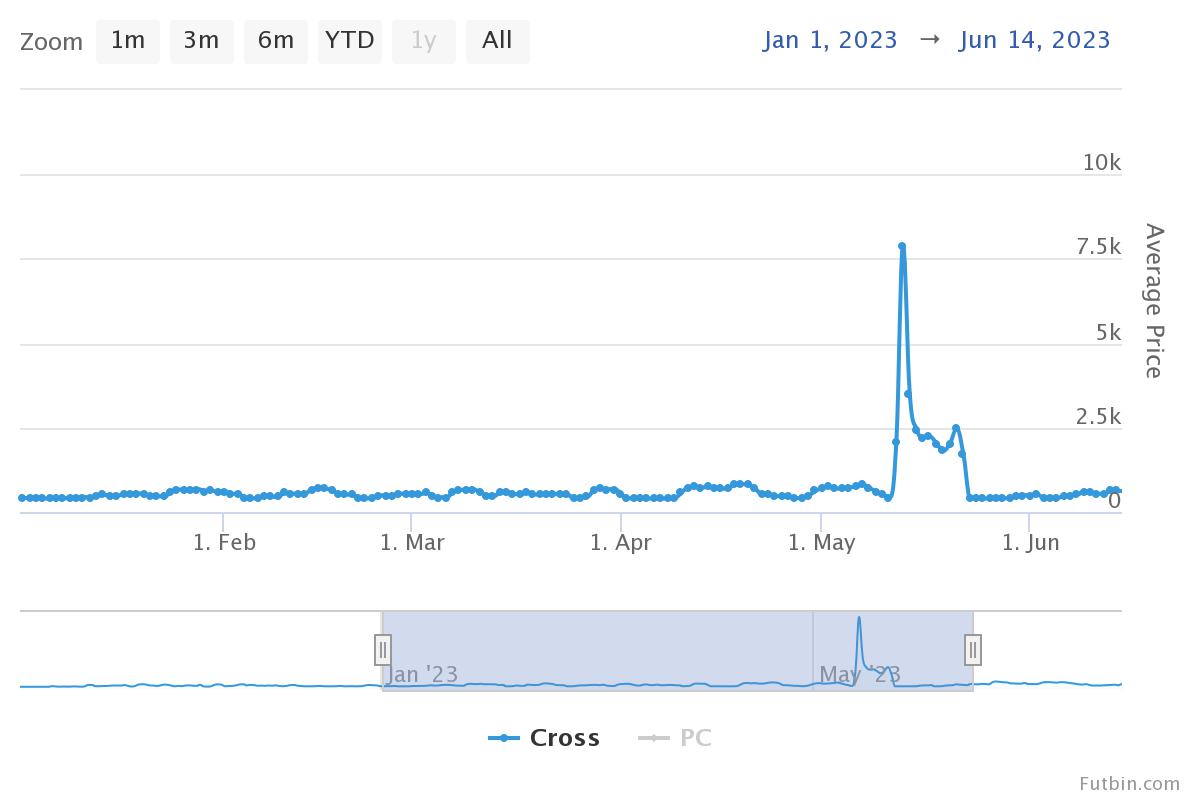
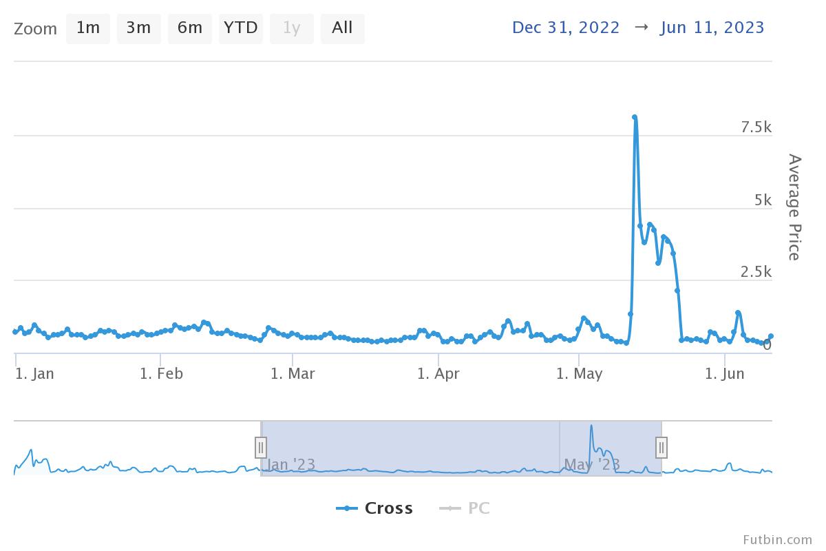

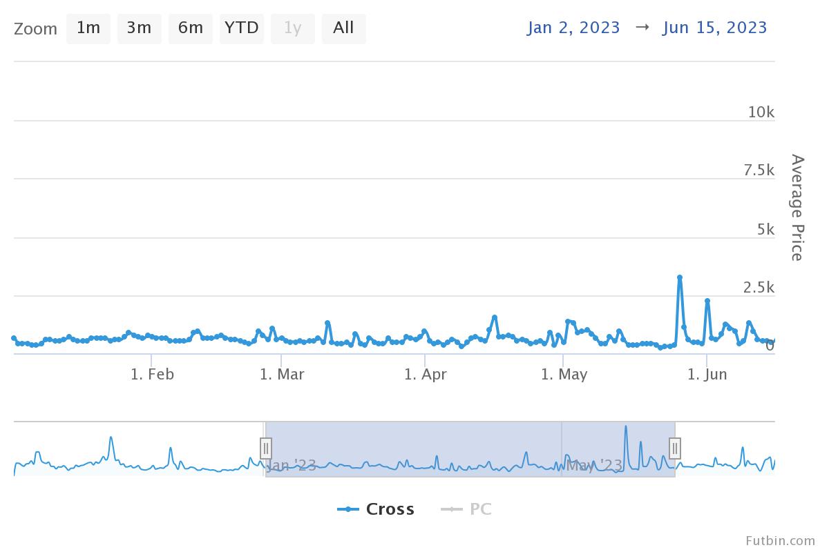
These figures were generated on July 26, 2023, on Futbin.com. The top row are prices for player cards Jovetić (left) and Lukébakio (right), the bottom row are prices for player cards Wind (left) and Thielmann (right).
I am not completely sure what exactly explains the initial price hike for the Hertha Berlin players beyond the eventual temporarily stable prices during which the objective was open. But I believe the price hike is a bit of an initial overreaction to the demand shock with a later quick convergence to the new equilibrium prices. I believe that this is caused by a quick increase in demand with a slower increase in the supply of these cards. I believe that it took the people who owned one of these cards a bit of time to realize that these cards just became more valuable and that it would now make sense to put these cards on the market to sell.
In any case, the Fifa 23 Ultimate Team market for player cards offers many fascinating episodes of quickly changing demand and supply and resulting price adjustments. If nobody has done so yet, perhaps someone should rigorously study this market and the economic forces at work behind it.
-
A nowhere near miss

I was involved in what was definitely not a traffic accident and it was my fault. Ok, let me try again. What I mean is that, while we were indeed far from having an accident, our actions were also not in equilibrium and that was my fault. I didn’t do anything legally wrong, I think, but the other person involved was right to be upset about my actions. In this post I will try to explain what exactly happened in game-theoretic terms.
The situation was this: I and another person were both approaching an intersection. I was on my bike, the other person in a car. I had a stop sign in front of me and she clearly had the right of way. I was fully aware of all this and I dutifully stopped on the fat white line. So, as I said, I didn’t do anything legally wrong. My opponent in this encounter, however, also stopped. And when she stopped, she stared at me accusingly, then shook her head and eventually drove on. Why did she stop and why was she mad at me? Well, because I didn’t look at her. No, she was not offended or anything like that. The problem with me not looking at her was that she didn’t know whether I had seen her. And she was worried that I will, like many bicyclists in Graz (where I live), think that I am alone on the road and ignore the traffic signs and just keep going. She didn’t want to run me over, so she stopped.
My lack of looking at her and, thereby, not openly acknowledging her presence meant that we did not have common knowledge of the fact that I did know that she was there. I knew that she was there and she, of course, knew that she was there, but she did not know that I knew that she was there. It feels good writing things like that. Anyway, the upshot was, that she, being apparently a very considerate and careful driver and being unsure of what I would do, stopped to avoid running me over. Her action was definitely caused by me not looking at her. If I had looked at her, she would not have stopped, as she would have seen that I had seen her and, thereby, most likely rightly, assumed that I will stop.
In the end, I guess one could say that we did not play the equilibrium action profile, which would have been for me to stop and for her to breeze through the intersection. My lack of looking at her made her stop when she didn’t need to. She lost valuable time because of me and I fully understand her anger.
-
Predicting the outcome of the world cup

There are many teams that can win the upcoming football world cup in Qatar and nobody can at this point know which of them will win. The best one can do is to provide probabilistic predictions. I will here explain how one can check the correctness of probabilistic predictions and will use this to argue that, quite possibly, the best predictions are those that one can derive from the sports betting market. My argument is based on using a large data set of betting odds to test the so-called efficient market hypothesis.
The outcome of one game (or one world cup) is not enough to test the predictive power of probabilistic predictions. Suppose you predict that, say, France beats Australia with probability 2/3 and I predict that France wins with probability 1/3. Suppose Australia wins. Was I correct and were you wrong?
It is essentially impossible to meaningfully test a single probabilistic prediction (unless you predict probabilities of, or very close to, zero or one), but you can test a (large) set of predictions. Betting markets provide such a set of predictions in terms of the betting odds that arise from people betting on the various outcomes of games.
Betting odds are the equivalent of prices in stock markets. They are also determined by supply and demand. But because they are a bit different from prices, I should probably briefly explain how they are typically determined by the betting companies. A football game between teams A and B can end in three key outcomes: team A wins, a draw, or team B wins. You can bet on any of these three events. In fact, you can bet on a lot more, but I will not pursue this here. When you are betting you are typically given odds. If the odds are
then this means that, if you put one euro on this bet and you win, you get
the odds for one game for the three events: team A wins, a draw, team B wins. Let me denote by
the amounts of money put on these three events. Then the betting company sets odds, for any event
from the set
as close as possible to
where
is the proportion of money that the betting company keeps, and is often around 5%. By doing so, the betting company has essentially no risk and simply makes around 5% of the total amount of money that was placed on bets, regardless of how the game ends.
If the odds that team A wins are
then
is the implicit probability that team A wins in the following sense: if
(The
for placing 1 Euro on this bet; and with probability
Let us now turn to the statistical analysis of these betting odds. I am using betting odds data for more than 200.000 professional football games from most of the major leagues in the world between 2006 and 2019 (downloaded from pinnacle.com in April 2019). I have chosen to focus on home team wins.
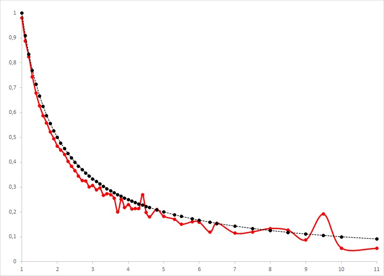
In the above figure I compare the actual observed win frequencies (fat line in red) with the implicit probabilities (dashed line in black) for all odds between 1 and 11 (on the x-axis). Isn’t it remarkable how close these two curves are? Look, for instance, at these two points: Of the 3138 games with betting odds of 1.2 with implied break-even probability of about 83%, the observed winning frequency is 82.3%. Of the 11045 games with betting odds of 2.2 and implied break-even probability of 45.5%, the observed win frequency is 43.2%. Note that the two curves come from entirely different data. The implicit probabilities are derived from the betting odds, which in turn, as I explained above, are derived exclusively from the betting behavior in the betting market. The observed win frequencies are derived from counting how often teams win their football games. Two entirely different things. And yet, they match almost perfectly. One could say that the implicit probabilities derived from the betting odds are really well calibrated: they are great estimates of the actual winning probabilities of, in this case, the home teams in football games.
This idea is, in fact, an implication of the so-called efficient market hypothesis: the hypothesis that market-prices aggregate all information that people may have, and, thus, deliver the best estimates for the underlying probabilities.
There are a few caveats to what I just wrote. Looking at the above figure we note that it is in fact true that almost all actual winning frequencies are below the implicit break-even probabilities. This derives from the fact that the betting company keeps its
-proportion (typically around 5%) and could easily be adjusted. This also means that for all these odds if you had put one euro on every single one of these games you would have lost money.
But what about the few odds for which the implicit probability is above the observed win frequency? This happens for 6 out of 53 odds. It happens for odds of 4.4, 4.8, 6.5, 8, 8.5, and 9.5. Does this mean that we should bet on games with these particular odds in the future and, doing so, will make money on average? Does this contradict the efficient market hypothesis?
I don’t think so. With 2292 games in total there are not that many games with these betting odds in the data set. For the two betting odds of 4.4 and 9.5, for which the observed winning frequency is more clearly above the implied break-even probability, there are only 26 and 94 games. Even if the true winning probabilities are less than or equal to the implied break-even probabilities, one can relatively easily get higher observed win frequencies for at least some betting odds purely by chance. For the statisticians among you, one cannot reject the null hypothesis that all true win probabilities for all betting odds are less than or equal to the respective implied break-even probabilities with the given data (p-value of 0.189). Let me know if you want to know what statistical test I used.
So, we cannot reject the null hypothesis, implied by the efficient market hypothesis, that the betting odds are well calibrated. Does this mean that one couldn’t potentially produce better probabilistic predictions? Does this mean that the efficient market hypothesis is true? No. This is only one possible test of the efficient market hypothesis, which not only states that implicit probabilities should be well calibrated, but also that they include all the information that is available about the games out there in the world. There is a sense that we know that this is not true. Occasionally, there are games that are rigged. This means that there are some people who know how these games will end, and this information is often not reflected in the betting odds. But, on the whole, and this is still a bit of a leap of faith, I believe that it is hard to come up with more accurate probabilistic predictions of how football games end than those derived from the betting market.
Who will then win the World Cup? According to the betting odds of the 9th of November (from oddschecker.com), Brazil is the favorite with a win probability of 23.8% (betting odds 4.2). This is followed by Argentina with 16.1% (betting odds 6.2), France with 14.3% (betting odds 7), England with 11.4% (betting odds 8.8), Spain with 11.1% (betting odds 9) and Germany with 8.3% (betting odds 12). Saudi Arabia and Costa Rica have the lowest chances of winning with 0.1% each (betting odds 1000). However, these probability predictions can change at any time if there is relevant new information. For example, if Messi were to get injured, that would immediately change all betting odds and therefore all probability predictions. The betting market processes this information incredibly fast.
-
What game theory can and cannot do

Game theory offers a formal language to study strategic interaction. Is it possible to use game theory to predict the outcome of every possible strategic interaction in the real world? Of course not. There are, at least, two problems. One is that game theory when applied to some real-life strategic interaction, needs to be empirically well informed. The game theorist needs to know who the relevant decision makers (the players) are, what they can do (their strategies), and how they care about the various outcomes (their payoff function). The game theorist also needs to know what the relevant decision makers know about each other, what they know about each other’s motives, and what they know about what others know (the players’ information). Only if the game theorist knows all this, or has a good first-order approximation of all this, can they begin to try to come up with a prediction for the strategic interaction at hand.
For instance, it may be possible to use game theory to predict the outcome of the war in Ukraine for a very well-informed game theorist, but it is certainly not possible for me, as I wouldn’t even know where to begin modeling this conflict as an empirically reasonable game. If you would ask me what I believe the outcome of this conflict would be, I would first be asking you questions. And as you would probably not be able to answer most of them, I would not be able to give you a prediction. For a good game theoretic prediction, you would, therefore, need a game theorist teaming up with someone who has the appropriate empirical knowledge. That is why I, in this blog, tend to write about real-life strategic interaction, typically of a smallish nature, that I have personal experience with, so that I can be reasonably confident that I will make the appropriate assumptions when I build my game theoretic model. After all, I am no expert on any particular real-life strategic interaction, I am an expert (if at all) on how to formally model strategic interaction and how to mathematically “solve” these models.
But there is also a second problem. Suppose the game theorist does have a good idea of what the right game is for the real-life situation at hand. The game theorist may still struggle to come up with good predictions. Consider tic-tac-toe. You know, the game with crosses and circles. There is a 3 by 3 grid and players alternate one player placing crosses and the other circles in this grid. The first of the two players to have managed to place three of their symbols in a row, horizontally, vertically, or diagonally, wins (and the other player loses). If neither player can do so, it is a draw. Suppose both players want to win. With this knowledge, the game theorist has, one would think, all they need to be able to write down the appropriate game. Ok, one could argue, and in that case what I will write in a moment is just a version of the first problem, that the game theorist still doesn’t necessarily know how much the players understand the game. In fact, this is the problem that I wanted to come to. A game theorist would be able to come up with predictions for this game. This is a relatively simple game, with the feature that both players could, in principle, at least guarantee themselves a draw. So, Nash equilibrium, for instance, would predict that every such game ends in a draw.
I want to argue that, first, this is, of course, empirically wrong, yet, second, this is still very useful knowledge and helps us explain something about the world.
Ok, first, of course not every real-life tic-tac-toe game ends in a draw. I have often seen kids play this game and observed that sometimes one child and sometimes another wins this game. I have also involuntarily watched a grown man one row in front of me on the airplane repeatedly losing tic-tac-toe against the computer in the easy setting of the tic-tac-toe program on the back of the seat in front of him.
As a game theorist, you would really need to know a lot more than the players, strategies, and payoff functions, to be able to predict all these outcomes correctly every single time. You would probably need to know, what Jeeves (from the P.G. Wodehouse books – if you don’t know about this you are missing out), would call the “psychology of the individual.” I like this term because it stresses the term “individual.” It would not suffice to know something general about psychology, you need to know the individual, as obviously not everyone plays the game in the same way. In fact, you need to know even more, you need to know how the players feel at the moment and how motivated they are and what they know about and what they have learned about the game so far, and probably much more, to have any hope of coming up with a good prediction of their behavior every single time.
I believe that there are cases of real-life strategic interaction, such as some random kids playing tic-tac-toe, that are essentially unpredictable. This does not discourage me from using game theory. Why not? I still think the Nash equilibrium prediction (other ideas based on the elimination of dominated strategies would also come to the same prediction) is useful. It explains why we do not have high-prize competitive tic-tac-toe tournaments. If we had such tournaments, the incentives to win in these, given the high prizes, would be very high. People would have a strong incentive to learn to play this game well. Such learning will eventually, at least in simple games such as tic-tac-toe, lead to Nash equilibrium behavior. As this behavior is finally always the same it would be very boring. Nobody would come and watch a tic-tac-toe tournament where every game ends in a draw and the winner has to be decided by coin flip every single time.
While the Nash equilibrium prediction would, thus, be empirically wrong in many real-life settings and probably also in many potential lab experiments, it is still useful to understand something about our world.
-
Strategic sports

Not all sports have strategic elements. There is not much strategizing in the 100-meter dash. You just run as fast as you can. That’s all there is to it. I have also never heard of a 100-meter racer employing a strategy coach. Mental coaching, yes, physical coaching, of course, yes, but strategic coaching, no. It is just not necessary. All they would say is: “Try to run as fast as possible” and you don’t need to pay someone to give you this kind of advice. There is probably also not much strategic concern in the long jump, the high jump, pole vaulting, and javelin. I guess there is little strategic thinking in most of athletics. But there are also lots of sports, even within or close to athletics, that do have a substantial element of strategic consideration.
Take the so-called “sprint” race of track cycling. The main rules are as simple as those of the 100-meter dash. To quote from a reliable source, “two riders race off over three laps to see who is fastest.”
The first time I watched such a race at some Olympics, I expected, now I know somewhat naively, that the race would be simply a cycling version of the 100-meter dash. The two cyclists would come out flying and race as fast as possible until one of them crosses the finish line. This is not what happens. What happens is that at the crack of the starting pistol essentially nothing happens. The two racers amble off, almost going as slowly as possible. You can see this for yourself. The front “racer” meanders around, sometimes veering left (or down the track, as the track is slanted) and sometimes veering right (or up the track). The other rider carefully mimics these movements. Sometimes they almost come to a standstill. This goes on for quite some time and all this time the front “racer” constantly turns their head to look back to check up on their opponent. At some, ex-ante unclear, point in time, one of the two, finally and suddenly, starts to pedal as hard as possible, with the other racer trying to catch this moment and trying to start pedaling as hard as possible as well. Finally, the race deserves its “sprint” name.
Why don’t we see what I expected to see, that both cyclists race off as fast as possible from the start? Well, the reason is that this is simply, in the language of game theory, not a Nash equilibrium. When your opponent does race off as fast as possible, you do not want to do the same. What you want to do, this is the best response behavior as game theorists would call it, is that you go fast, yes, but behind the other cyclist, in their slipstream. Because of the physical advantage that this gives you, you do not have to exert quite as much effort as the front cyclist does, and after you have been in the slipstream for about two of the three rounds, you can come out of it with an even higher speed and overtake your opponent just before the finish line. More often than not, with that strategy, and if your opponent just races as fast as possible, you will come out on top.
Because of this, nobody just races off like that. I wonder if the current way the race pans out is what the original inventors of the sport had in mind. I wouldn’t be surprised if the original inventors were quite as naïve as I in thinking that the two cyclists would simply race as fast as possible. I could imagine that, for a while, the cyclists would even have done this. Imagine two very unevenly matched cyclists. The stronger of the two could then probably win simply by going as fast as possible. The slipstream effect is not THAT strong. It only becomes an issue, I would think, when the two cyclists are pretty similar in their athletic ability, and, thus, only when the sport becomes quite competitive. I couldn’t find any good source for the history of this event, but there are some indications that it took a while for the currently observed behavior to unfold. First, the sport has seen occasional rule changes: at some point, rules were added that cyclists are not allowed to stop completely or go backward or put their feet on the floor. These are indications that a Nash equilibrium had gradually established itself (because perhaps of a higher degree of competitiveness and a certain (slow?) learning) in which the competitors did that. The rules were then introduced because otherwise, the sport would have become too boring. Perhaps there were races that instead of the minute or so that a race should last, took hours to complete, because none of the racers was willing to start the race properly, thinking they would lose the advantage by doing so.
Second, another sprint event, the individual pursuit, was introduced, quite a bit later if I understood this correctly, that can also be seen as a rule change. In this case, however, with both kinds of races remaining (somewhat) popular. The individual pursuit is very much like the sprint race, except that the two cyclists start from opposite positions (half a track apart) from each other. Slipstream effects cannot come into it now.
In any case, the sprint race is actually quite interesting to watch, mainly because it has interesting strategic considerations. I guess what we are seeing is pretty close to Nash equilibrium behavior. Moreover, this Nash equilibrium behavior is quite complex. As it also probably strongly depends on the relative strengths of the two competitors, it is also somewhat varied. You don’t get the same predictable outcome in every race. All this, I believe, explains why the track cycling sprint event has remained a (reasonably) popular and Olympic event, despite or perhaps even because it has such strong strategic considerations that seem in strong contrast to the perhaps originally intended pure athletic nature of the competition.



-
Subscribe
Subscribed
Have a WordPress.com account? Log in now.

