-
Meeting inside a crowded stadium without communication

Three of us have just been to Emirates Stadium to see a football game. We witnessed and participated in some interesting rational herding walking to the stadium, as I described in my previous post. But once inside, we had another game-theoretic problem. The problem was caused by the fact that we didn’t all have seats together. After a quick bite to eat at one of the food stalls inside the stadium before kickoff, we went to our separate seats without communicating how we would meet again at halftime. It didn’t occur to us at the time that maybe we should have talked about this. When we then got to halftime, when people started flooding back from their seats into the food stall area, I realized that we hadn’t arranged where we would meet, and I was wondering for a moment how we would manage to do so. The food stall area is huge. It goes all the way around the stadium, I believe. So where was I supposed to go?
I thought about it a bit, and realized that there is really only one place that sticked out, most likely not only in my mind, but quite possibly also in the mind of my family members I was trying to meet: the stand-up table where we had our food together and that was also the last place at which we were together before the game started. And this is indeed where we found each other, pretty quickly, and without having to resort to communicating with our (Austrian) phones (that don’t work so very reliably in London).
In principle, we had a difficult coordination problem. We could have met anywhere in the stadium. And the stadium is huge and full of people. If I had thought for some reason that my family members would go to, say, Stand-Up-Table 157 (counting from the entrance, say), I should have gone there as well. If I had thought that my family members would all come to my seat, I should have waited for them at my seat. If I had thought that my family members would go to the entrance we came in through, I should have done the same. Game-theoretically, this situation is well described by a large pure coordination game in which all three of us have the same large strategy space (the set of all possible places we could meet) with payoffs such that we all get the highest possible payoff, say 1, if we all choose the same strategy, and, for simplicity, 0 otherwise. Such a game has as many (pure strategy) Nash equilibria as it has strategies. A Nash equilibrium is a strategy for each of us such that if the others follow it, I also want to do so (and the same is true for the others). So, for every place that we could have met at, the strategy of going there is a Nash equilibrium strategy.
Contrary to popular belief, game theory does not generally predict (Nash) equilibrium play, even if the players are assumed to be extremely rational. In fact, even common knowledge of rationality does not imply equilibrium play. Common knowledge of rationality means that everyone involved is rational (which in turn means that everyone has clear goals and chooses actions that best achieve these goals) and that everyone knows that everyone is rational and that everyone knows that everyone knows that everyone is rational, and so on ad infinitum (as we like to say). We probably rarely have common knowledge of rationality in actual real-life situations of strategic interaction (as in our case here). But, it would, in any case, not imply that we would play an equilibrium. Common knowledge of rationality only implies that the outcome will be, what is called rationalizable. Without telling you what rationalizable strategies are, I can tell you that there are some games in which there is only one rationalizable strategy profile, and that would have to be a Nash equilibrium. But in coordination games the assumption of common knowledge of rationality yields the following prediction: anything is possible.
So, how did we manage to meet after all in these difficult circumstances? In some situations of strategic interaction there are strategies that Thomas Schelling called “focal points,” see the Wikipedia entry for a starting point. As you will notice when you read this entry, there is no generally workable definition of a focal point given. I have once attempted to provide such a definition of a focal point in a paper with Carlos Alós-Ferrer, but while I like it a lot, it is perhaps only partially satisfying. The idea is relatively straightforward, though. A focal point is a strategy (profile) that, among all other strategies, jumps out at all of you: it is specially earmarked, relative to all other options, in the minds of all the people involved. In our case, the table at which we had food together, and that was also the last place before we went our different ways to our seats, was so earmarked in all our minds. And given this earmarking, we all followed the strategy of “go to the place you have collectively earmarked.” This strategy only works if you indeed earmark the same thing. In reality, many situations lack such a clear focal point, with the implication that you do not manage to meet, or at least not quickly, or not without further communication. One of the problems with the theory of focal points, is that it is a bit difficult to state when and when not it should work. But it did work in our case, and I was happy about that. One could say that because of Newton we did not float into space, and because of Schelling we managed to meet.
-
Rational Herding to get to Emirates Stadium

Three of us have just been to Emirates Stadium to see the Arsenal football club’s last friendly match before the new season starts. Some of us had been to the Arsenal Shop at the Stadium, and some of us had a stadium tour before, but none of us had yet seen a game. Our plan was to take the tube, the Piccadilly line, to Holloway Road, as we had done in the past on our previous visits to the area. We had plenty of time. We aimed to be there about an hour before kickoff. We were not alone on the tube, there were plenty of people in Arsenal shirts. When we got closer to the stadium, the train driver announced that the Holloway Rd tube stop was closed and that the train would not be stopping there. I believe this was due to it being a pretty small tube station with fairly narrow exits and some lifts not working. It may be that they close Holloway Rd tube station whenever there is a game on. Nobody on the train panicked and we simply readjusted our plan to get off the train at the next stop instead, at a stop aptly named Arsenal. I believe that even the train driver was a bit surprised, although not unduly, when he announced that the Arsenal tube station was also closed, and we would all have to wait to get off at the tube station after that: Finsbury Park. Again, nobody panicked, but there were some more animated conversations on the train now. By the way, this is not a blog post about panic, nobody panics at any point during this story. But something interesting did happen. And I am getting to it.
We arrived at Finsbury Park tube station, the doors opened, and we made our way to the exit. For a while, there was only one useful direction we were told to take by the “Way Out” signs. We, and everybody else, followed these signs. We were a bit slow for some reason and were perhaps some of the last people in the crowd to get out of the station. At one point the crowd, which was mostly just ahead of us, got to an intersection, with multiple possible paths leading out. The whole throng was heading in the same one of the three possible directions. I feel there were three possibilities, but maybe there were only two. In any case, the throng then slowed down a bit. It takes a bit of time for people to get through the tube barriers – to “tap out” with their Oyster cards (or credit or debit cards). So, we slowed to almost a standstill, which allowed us to consider our options. Should we follow the throng, or should we aim for one of the other exits, that nobody was using? We were weighing the pros and cons, given the limited information we had. Another exit would be quicker as there would be no congestion. But we were not sure where this other exit would take us. Some tube stations in London have exits that are quite far from each other with roads and buildings between them that would be hard or at least time-consuming to cross. It would also take us some time to get our (Austrian) phones (if we even had any reception) to help us with the directions at a tube station. We felt that all these other people, almost all of them going to the game, with all their clearly visible Arsenal paraphernalia, probably knew what they were doing. At least some of them should probably know the quickest way from the inside of the tube station to the stadium. None of the others seemed much torn over the decision as to which of the two or three exits to take. So, in a matter of a few seconds, we decided to follow the throng through the somewhat congested exit it was taking.
We slowly followed the throng out of the station and then also along the roads. After a few turns and a few minutes of walking, I noticed that we passed another tube station entrance/exit. So did we all take the wrong exit after all? I am not 100% sure, and some people may have taken the exit that we have all taken because they really wanted to. After all, we were quite early and some of the Arsenal supporters may have wanted to go to a favorite pub somewhere in the vicinity before going to the stadium. But I do believe that many of us took what in hindsight we would consider the wrong route out of the station. Once I was back home I studied the Finsbury Park tube station map carefully. This is the nicest map I found, even if it is from 2016. There are three exits. The throng with us in tow left the station through the Wells Terrace exit (the one marked closed on this map, but it has reopened since 2016). The exit we passed later, actually we were going round clockwise, was the Seven Sisters exit in the south of the station, and south is where the Emirates Stadium lies. I also studied Google Maps for some time, and I am pretty convinced that it would have saved us some 5 minutes or so if we had taken the Seven Sisters exit instead of following the throng.
So, did we make a mistake? In hindsight, I guess, yes, but given what we believed at the time, we made the best decision. We believed that others knew better which the best exit to get to the Emirates Stadium would be, so we rationally followed the herd. Was our belief silly? No, I don’t think so. After all, we had almost no information to begin with as to which exit would be best. And it seems reasonable that we should at least attach a higher probability of the throng going through the right exit than the wrong exit. Should we now be shocked that the exit we all took was wrong after all (for most of us anyway)? No, we probably should have realized that there is no 100% guarantee that the throng did go through the right exit. After all, many of the eventual spectators of the game were not the usual Arsenal supporters – we, for instance, not being registered members of Arsenal would not normally be able to get tickets to a league game. Moreover, I believe that people usually get off at Arsenal tube station and not at Finsbury Park. Many people in the throng were, therefore, probably in a similar situation to us, they did not know which the best exit was and were also hoping that the people in front of them knew more than they did. What about the first few people out of the tube station? Well, maybe they also did not know perfectly and made an educated guess, which turned out to be wrong. Maybe, they had a different goal. Maybe they were the first out because they wanted to get their beer in their favorite local pub as quickly as possible and their favorite pub wasn’t quite on the fastest way to the stadium, but others behind them did not know that.
All in all, I believe that we found ourselves in a situation that is well described by the rational herding models that started with the 1992 paper “A Theory of Fads, Fashion, Custom, and Cultural Change as Informational Cascades” by Bikhchandani, Hirshleifer, and Welch, see also my previous post on rational herding on the Autobahn. One of the main points of these models is that, even though everyone in the model is rational, sometimes, ultimately, everyone makes the wrong decision, as it seems we have done in this case.
-
A strategic dilemma in the 2024 Olympic Women’s Road Race

When Kristen Faulkner made her move to start to get ahead of a four-women group of cyclists, the remaining three had an interesting strategic dilemma. The outcome of the dilemma was that they let Kristen Faulkner go without trying to catch up with her. Kristen Faulkner won Gold, and two of the remaining three won silver and bronze. If the remaining three had collectively decided to push to follow Kristen Faulkner, I believe one of them would have won Gold instead. So why didn’t they?
Lotte Kopecky, the eventual bronze medalist, when asked what happened after Faulkner’s move, said: “It’s a move you can expect. You know she’s going to do it. Then the three of us look at each other, so we are just stupid.” And Faulkner after being asked about it said: “I don’t know – you tell me what happened.” Both of these according to NBC.
I think the outcome of this situation would have been different if there had only been three in the leading group, and therefore only two cyclists to chase Faulkner. The fear of losing out on a medal may have been important in this strategic problem. I don’t know a whole lot about cycling, but I am aware of the slipstream effect. I believe the problem that the three chasers had was this. They all knew that they should now chase Faulkner, but none of them wanted to be the front chaser. Because the front cyclist has to work much harder than the cyclists behind her, due to the slipstream effect, and would most probably have eventually been overtaken and would, thus, most likely have lost out on a medal. If, on the other hand, the three don’t chase, then everyone has a decent chance of winning one of the two remaining medals.
One of my aims with my blog posts is to demonstrate that game theory is much more than the prisoners’ dilemma – many interesting strategic situations cannot be reduced to the prisoners’ dilemma and require some other approach taken from the incredibly versatile toolkit of game theory. But, the problem that the three remaining cyclists had that Faulkner left behind in her race to the gold medal, is very close to the prisoners’ dilemma. The three cyclists had the choice to race off to follow Faulkner. If any of them had chosen to race off to follow Faulkner, the other two would have had a good chance to win the gold medal. But crucially, the one that races off first, probably does not have a good chance to win gold, in fact she might have a good chance to come fourth. Because of this, none of them followed Faulkner.
Could they have done better? Yes, possibly. They could have come to an agreement that they alternate the leading position in the chasing group at reasonable intervals. I guess, this is what they were trying to do when they were looking at (and talking to?) each other just after Faulkner raced off. But it is not easy to come up with such an agreement on the spot and in a short amount of time. And it doesn’t look like they managed to do so.
-
Ex-post probability assessments from expected goals statistics

The expected goals statistics (xg) in football/soccer games have been around since 2012, but I have only really started to notice them properly in the last few years. They are an interesting attempt to quantify and objectify randomness in football games. In this blog post, I want to explain how one could use these statistics to compute probabilities of the various results of a game after the game was played.
Computing probabilities of how a game could have ended after it was played does perhaps seem a bit silly. After the game, we already know how it ended. However, it could be quite relevant to a sober judgment about a team’s performance. Sometimes journalists heap praise on a team and its manager after a game that ended with a tight 1:0, where the opposition had plenty of chances that they did not take; sometimes journalists condemn a team and its manager for a game lost with a wonder strike in the last minute. I often feel that there is generally a lack of a proper appreciation of the randomness in football games.
Of course, you could ask whether there is any randomness in football at all. One can take the view that everything is deterministic and just a question of (Newtonian I think would suffice) physics. But I would think that most people would agree that there are some factors that nobody can control and nobody can completely foresee (even if they understand physics). An unexpected sudden gust of wind might make the difference between a long-range shot hitting the bar so that the ball goes in, or hitting it so that the ball stays out. An invisibly slightly wetter patch of grass might make the difference between a sliding tackle getting to you in time to take the ball off you, or just falling a tad short of that.
Once you allow for some such randomness, the next question would be how one should quantify such randomness. In fact, can we quantify it in terms of probabilities and even if we can, would we all come to the same conclusion? There are some instances of randomness that researchers (on the whole) would refer to as objective uncertainty, also often called risk. A good working definition of objective uncertainty (or risk) would be that it is such that most people assign the same probabilities to the various events (events = things that can happen). Think of the uncertainty in a casino in games such as Poker, Roulette, Blackjack, Baccara, or Craps. Most people would agree that the chances of the ball in roulette coming up, say, 13, is 1/37, because there are 37 numbers (0 to 36), symmetrically arranged around the roulette wheel. If someone told me that they feel lucky and think that the probability that their number, say 13, will come up is 50%, I would even believe that they are just wrong.
Outside the casino, it seems that most of the uncertainty we encounter is not objective in this sense. Uncertainty is often in the eye of the beholder, as people like to say. This is even true in the casino at times. If you have two aces in your hand playing poker, your assessment of you winning this round will be different from that of your opponents, who don’t know which cards you are holding. Similarly, someone who has observed the weather over the last 48 hours would probably make different weather predictions for the next day than someone who has not done so.
There is a deep philosophical debate in the literature (google the common prior assumption) as to whether we should model different individuals’ different probability assessments over some events as deriving exclusively from them having seen different information, or whether individuals could also sometimes be modeled as just having different beliefs about something – period. Luckily, this debate is not hugely relevant to what I want to discuss here. But I do believe that it is just empirically correct to say that different people would often quantify randomness differently (for whatever reason). You might suspect that some people don’t quantify uncertainty into probability at all. Probably true, but one has to be careful. People might not be able to tell you what probability they attach to certain things, but they might behave as if they do. I also don’t want to get into this either, though.
What I wanted to say is that I believe that football games have uncertainty that is not typically considered objective. Ask two different people (perhaps ideally people who bet on such things) about the chance of how a game would end and you will probably get two different answers. But I do like attempts to objectify the randomness in football games. And the xg approach is a pretty good attempt. As far as I understand, see again this post, an xg value for any chance at goal in the game is computed using a form of (probably logit- or probit-like) regression given a large data set of past shots, where shot success is explained with variables such as distance from goal, the angle of the shot, and many other factors. Personal characteristics do not seem to be used. This means that the same chance falling to Kylian Mbappe or a lesser-known player would have the same xg. We might come back to that later. [Actually, now that I am finished with this post, I see that we won’t. A shame.]
I want to get to one example that I will work through a bit, to eventually come up with what I promised at the beginning, an after-the-game assessment of the probabilities of how the game could have ended. Let me take the, for Austrians, slightly traumatic experience of the recent round of 16 game between Austria and Turkey at the 2024 European championship in Germany, which Austria lost 1:2. I found two good sources that provide an xg-value for this game: the Opta Analyst and a website called xgscore.io. Both provide xg-values for the two teams for the entire game: this is the sum of all xg-values for each goalscoring chance. The Opta Analyst makes it an xg of 3.14 for Austria and an xg of 0.92 for Turkey (when you click on the XG MAP in the graphic there) and in the text they make it: “Austria can consider themselves unfortunate, having 21 shots to Turkey’s six and recording 2.74 expected goals to their opponent’s 1.06.” Xgscore.io finds an xg of 2.84 for Austria and an xg of 0.97 for Turkey. So even they do not all agree.
An objective assessment of expected goals for each team is not quite enough yet to compute the probabilities of how the game could have ended. I need an assessment of not only the expected goals but also their variance. In fact, two teams with the same xg of 1, could have a very different distribution of goals scored. One team could have had an xg of 1 because they had one chance and that one chance had an xg of 1; perhaps it was a striker getting the ball one meter in front of goal with the goalkeeper stranded somewhere else on the pitch. Then this team would have scored 1 and only 1 goal, and that with certainty. Another team with the same xg of 1 could have had two chances that both had a 50% of going in. This team could have scored 0, 1, or 2 goals, with 0 and 2 goals 25% likely and 1 goal 50% likely.
I don’t think that Opta (or any other source) regularly provides the xg details for each goal-scoring chance that I would need to compute these distributions. But for the game Austria versus Turkey, I can get a sense of these distributions from the XG MAP provided on the analyst.
Let me simplify and take an xg of 3 for Austria and 1 for Turkey. I will now calculate the probability distribution of the various outcomes of this game under two different scenarios. In both scenarios, I assume that Turkey had two (stochastically independent) chances, both with a 50% likelihood of success, a 0.5 xg. The two sum up to one. This makes the number of goals scored by Turkey, call it X, a binomial distribution with n=2 tries and a success probability p=0.5. In reality, Turkey had 5 or 6 chances, with all but two of them rather speculative efforts – see the XG MAP. In the first scenario, I assume Austria’s xg of 3 is decomposed into six (stochastically independent) chances with an xg of 0.5 each. This is not quite correct, but also not a terrible approximation of reality. This means the number of goals Austria scores, call it Y, is also binomial with n=6 and p=0.5. All I need to do now is to compute the probabilities that X>Y (Turkey wins), X=Y we have a draw, and X<Y (Austria wins). I asked chatgpt to do so; it does it correctly and provides not only the results but also the various steps of calculation. In this first scenario, I got a roughly 3.5% probability of Turkey winning, an 11% probability of a draw, and an 85.5% probability of Austria winning.
In the second scenario, I keep Turkey the same, but I now assume that Austria’s goals scored Y is binomial with n=10 and p=0.3. That means Austria had 10 chances with xg values of 0.3 each. Again, not quite correct, but also not a terrible approximation of reality. With chatgpt’s help, I now get a roughly 11% probability of Turkey winning, a 12.6% probability of a draw, and a 76.4% probability of Austria winning.
It is interesting to see how much of a difference there is in the two scenarios. If I had the full data for this game I could compute the probabilities more accurately, which would be a bit harder because each goal-scoring chance will typically have a different xg value and the total number of goals scored by each team is not simply binomial. But with some computing effort, the various probabilities could still be calculated. I would like it if Opta (or any other source) were to provide these after-the-game winning probabilities induced by their xg statistics.
These after-the-game probabilities could now be compared with the before-the-game probabilities implied by the betting odds. I found betting odds for Austria vs Turkey here. In my notation, these are 2.05 for Austria winning, and 3.4 each for a draw and for Turkey winning. These translate into probabilities of 45.33% that Austria wins, 27.33% for a draw, and 27.33% that Turkey wins (I am making some assumptions here, ignoring the commonly observed favorite-longshot bias).
This does not mean that the betting odds were wrong, of course. It only means that, in some sense, Austria positively surprised the “market” in the game by producing a probably higher-than-expected xg-value, while in another sense, they negatively surprised the market by not winning.
So, assume that the xg-scores are indeed a good way to objectify the randomness of what happens in a game. Having detailed xg information, for every goal attempt, would allow us to compute objective probabilities for all possible ways the game could have ended. While I would very much like to see these after-the-match probabilities reported, and to see them used for a sober judgment of a team’s effort in a game, I also know that there is something we ignore when we do so. All this is under the assumption that the game would have been played equally irrespective of whether some of the earlier attempts at goal were successful or not. This is, of course, unrealistic. I, for instance, had the feeling that England tended to play better and with more urgency, creating more chances, when they were behind in a game than when they were in front or drawing. A team’s game plan is, generally, likely conditional on how the game unfolds. The randomness entailed in these game plans, however, is much harder to quantify.
-
The Euro 2024 betting market

During the recent European football championship, I recorded betting odds of winning the competition for all teams. I tried, and mostly succeeded, in recording these odds after every game from a website called oddschecker.com who say that they always report the best (that is highest) available betting odds across all sports betting providers. Email me if you’d like me to send you this data. One can think of sports betting markets as toy financial markets. In this blog post, I explore this toy market through my self-collected data set and see what insights we can glean from it (assuming glean means what I think it means).
I like to record these betting odds (not quite as on oddschecker.com) for an event (for instance that England wins the competition) as a number o that is the Euro amount you will receive for every Euro you place on this bet if the event turns out to be true (for instance that England wins the competition) – otherwise you lose your Euro. Betting odds are essentially determined by supply and demand, just like stock prices, as I explain in more detail in this previous blog post. I thought I would here, however, translate these odds into something more akin to a stock value. For every team, we can consider an asset that would pay out € 1000, say, in the event that this team wins the whole tournament. The value of such an asset at any point in time is given by 1000/o, because this is how much money you would have to place on this team to receive € 1000 if that team wins eventually. By the way, 1/o can also be seen as the break-even probability, of the event that this team wins the tournament, that would make you as a bettor/investor indifferent between betting on this team or not. If your subjective probability assessment of this event exceeds 1/o you should bet on this team, if not you should not (see the Appendix for why you “should”).
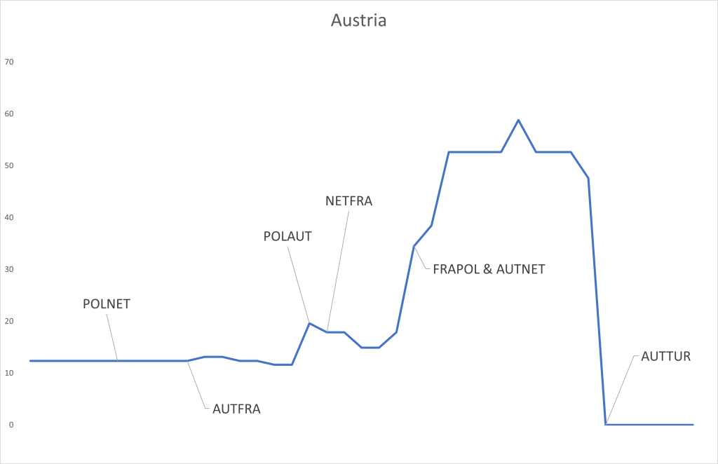
The above graph shows the value of this asset for Austria winning the competition. I have marked when certain games, most relevant for Austria, occurred. This asset “Austria” started before the tournament began with a value of around € 12,3 (because the betting odds were 81). This means, recall, that the “market” gave Austria a 1,23% probability of winning the competition at this time. When Austria lost to France 0:1 something remarkable happened: the value of “Austria” did not change. This means that the market expected some such result and performance from Austria, the result did not surprise one way or the other. It did not make the market think of Austria’s chances having improved, nor that their chances were diminished. My reading is that while a loss should have diminished the market’s assessment of Austria’s chances to win the competition, the otherwise solid performance in that game counterbalanced this. When Austria beat Poland 3:1 the value of the asset “Austria” went up to about € 19,6, the market now gave Austria a higher chance of winning the competition after this win. There are smaller changes in the value of this asset along the way, based on certain results and performances in other games, but when Austria then beat the Netherlands 3:2 and France drew with Poland 1:1, making Austria top of their group, the asset “Austria” went up to (after some little while – oddschecker may not have been quick enough with their updates) € 52,6 (giving Austria a 5,26% chance of winning the tournament). The next and last big change happened when Austria lost to Turkey in the round of 16 and the asset’s value went to zero.
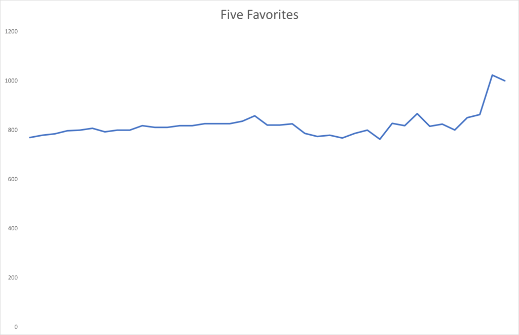
I find it interesting to look at the total value of the five favorites to win the tournament to begin with: England (odds of 5), France (5,25), Germany (6,5), Portugal (8), and Spain (10). The total value of these five assets (as shown in the graph above) started at € 769,3 (the market giving it a 76,93% chance of one of these teams winning the competition). This value changed remarkably little throughout the tournament, rising to a peak of € 866,7 after France beat Belgium in the round of 16, until before the final when there were only favorites left. [Btw, note that all five of these favorites went to at least the quarterfinals, and if one of them lost a game then only against another favorite.]
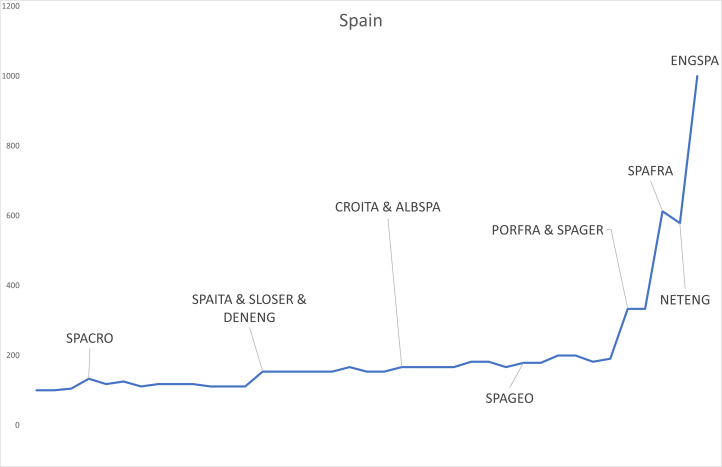
Let us, finally, look at Spain, the eventual winner of this tournament. In the graph above, I marked mostly those games that Spain was involved in. Spain seems to have gradually and consistently surprised a bit, or at least their market-perceived chances of winning the competition and, thus, the value of the asset “Spain” steadily increased over time. It started at a value of € 100 and reached a value of € 613 after Spain beat France in the semi-final, then briefly went down to a value of € 579 after England beat the Netherlands to reach the final – I guess this means that England was deemed by the market the more difficult opponent – before Spain finally won the tournament and the asset “Spain” paid out € 1000.
Appendix
When I said earlier that “[i]f your subjective probability assessment of this event exceeds 1/o you should bet on this team” I do mean that you should. Let me clarify. First, I think your carefully considered subjective probability assessment of any event should essentially never exceed its odds-induced break-even probability of 1/o, so you should never bet (see my point further below). But if it did happen that your (carefully considered) subjective probability exceeded 1/o then you should bet on this event. This is so because you “should” be risk-neutral. This in turn is so because the randomness in one such bet on a sports game is most likely idiosyncratic, I mean statistically independent from anything else that goes on in the world. It is, especially, most likely stochastically independent of the financial market. In the language of finance, any such asset based on sports bets has a CAPM beta of zero, where an asset’s beta is a measure of its correlation with the world financial market portfolio. Moreover, there are millions of such bets available, all independent from the financial market and most likely all more or less independent of each other. This means that if you put a small amount of money on any bet with a positive (carefully considered) subjective expected value, you would (in your carefully considered assessment) make a positive amount of money essentially without risk, because of the law of large numbers. Ok, this is assuming that you find many such bets, which maybe you shouldn’t be able to.
My subjective probability of any event I could bet on is essentially always lower than its break-even probability 1/o. This is for two reasons. First, I to a large extent believe in the efficient market hypothesis (https://en.wikipedia.org/wiki/Efficient-market_hypothesis), this is the hypothesis that all relevant information that anybody in the world (outside of insiders who are prevented from trading) could have about the value of a financial asset is reflected in the price of that asset. In the context of sports bets, all this information is hypothesized to be reflected in the betting odds. My belief in the efficient market hypothesis, especially for sports bets, is empirically somewhat justified for instance through some tests I made in a previous blog post. Second, you may ask how my probability assessment can be lower than the break-even probability induced by betting odds for all possible bets. Surely probabilities add up to one, and if one of my probability assessments is lower than its break-even probability then another will be larger. You are right that my subjective probability assessments sum up to one, but the odds-induced break-even probabilities do not! This is because the betting company keeps a small percentage share (around 5% or so) and all odds are a bit too small, so the break-even probabilities sum up to more than one. So, I never bet. While I would, therefore, advise most people not to bet (at least not in a big way), I am sort of glad that some do, because I do like to study the betting market!
-
Staying in Power with Minority Support

I once read somewhere something that Frederik the 2nd of Prussia, the “Great,” said to a general of his army. They were standing on a balcony overlooking the Prussian army and Frederik said something like “Isn’t it curious that we control them and not that they control us?” If you think about it, it does seem quite amazing. Thousands of people all do what one person wants them to do. And this, typically, not because all these thousands of people unanimously agree with their king’s commands. In many cases, one would imagine, many of these soldiers would personally rather not follow orders. Imagine going into battle, for instance, one of the purposes of having an army one would guess. Battles have a tendency to get people killed, often many people. It seems unlikely that many soldiers feel that it is in their personal interests to undertake an adventure that involves such a high probability of dying. Yet, they often do so. In this post, I try to explain with a bit of game theory, how one person can make a large number of people do what perhaps almost none of them want to do.
Before I do so, let me first admit that soldiers don’t always follow orders. In fact, the very same Frederik the 2nd of Prussia, as many other kings and generals through history struggled with the problem of desertion. This is evident from his detailed instructions (in Chapter 1 of https://friedrich.uni-trier.de/de/volz/6/text/) on how to prevent desertion. Generally, there are many strategies commanders of large armies use to forge and maintain a large fighting army. For instance, they aim to be charismatic and try to convince their army that they are fighting for a great cause, also potentially interesting topics for a game theoretic analysis. But here I want to focus on one, clearly always used, strategic device to maintain an army: the fear of punishment.
As one of the soldiers in the army, you follow orders even if you don’t like to, because if you don’t, something even worse happens to you. Your choice is typically not between going into battle or staying at home doing things you enjoy, but of going into battle or being jailed or even executed as a deserter or traitor. Given these limited choices, you “prefer” going into battle. But how is this punishment affected? Only through another command by the king that is followed by those whom he commands. What if they do not obey? Well, they then also face serious punishment, ordered by the king and executed by another set of soldiers. If they in turn also do not obey, another group of soldiers will be ordered to punish them. Often in such situations, it is unclear as to how many people are really behind the king, but some, a special guard with special privileges, for instance, may well be. There are many ways one could now model this situation as a game. I will here consider the perhaps simplest such game of interest, a large simultaneous move game with complete information. Both of these assumptions could and should be challenged, and, perhaps, we get there later.
The king’s strategy is simply to issue commands and then command some of the people to punish any who do not obey his commands. Let us fix his strategy, thus. Let us then look at the strategies of the soldiers, when, for instance, they are told to go and fight in a battle. To simplify, they can either obey or not obey. We have players, the soldiers, and their strategies in the game. Now we need the payoffs, as game theorists like to call them. First, we need to consider the various possible outcomes that can emerge in this game. Let us suppose that, as long as there are only a few soldiers who disobey, they simply get punished and the king’s wishes are executed regardless of some dissent. But suppose also that there is some threshold of the number of dissenting soldiers that when it is exceeded the king has no choice but to change his policy (not going into battle in the example we have used here). Let us call this magic threshold number k, and let us suppose for the moment that all involved know the value of this number.
We now need to specify how the soldiers like any such outcome that could arise. Let us consider two types of soldiers, one who is with the king and is happy to do what the king commands, and one who is not. A soldier who is not happy with the king’s commands might see the situation as follows. If they go into battle, they are pretty unhappy, say they get a payoff of -1. If they dissent and get punished and the army goes to war anyway, then they are even more unhappy and get a payoff of -c < -1. If there are so many dissenters that the army does not go into battle and there are no punishments, then they are happy and get a payoff of 1, say.
What about a soldier who likes to do what the king commands? Well, we could for instance, specify that such a soldier has a payoff of 1 when they go into battle, has a payoff of -1 if they don’t, and has a payoff of -c < -1 if he or she is punished (for some reason). Let us call the two types of soldiers “disloyal” and “loyal,” even though these are probably not the best terms. Their payoffs can then be summarized in the following two tables.
A loyal soldier less than k-1 others dissent k-1 others dissent k or more others dissent obey 1 1 -1 disobey -c -1 -1 A loyal soldier’s payoffs A disloyal soldier less than k-1 others dissent k-1 others dissent k or more others dissent obey -1 -1 1 disobey -c 1 1 A disloyal soldier’s payoffs A loyal soldier has a simple choice. For them obeying “weakly dominates” disobeying, as game theorists like to say. In the table, this can be seen by the fact that all numbers in the obey row are at least as high as the corresponding number in the disobey row. A loyal soldier will then just obey.
A disloyal soldier, however, has a more complex choice problem. They would prefer to disobey when k-1 others disobey also, thereby becoming the key additional dissenter that brings about the revolution. They are indifferent between obeying and disobeying when more than k others dissent, as then there is a revolution regardless of what they themselves do. But when less than k-1 others dissent, they “prefer” to obey, as obeying will not change the fact that they go to battle, and will only lead to them being punished for nothing, so to speak.
Call the proportion of disloyal soldiers p, some number between 0 and 1. Suppose for the moment that this proportion is commonly known: everyone knows it and everyone knows that everyone knows it and so on, ad infinitum, as game theorists somewhat pompously like to say. Suppose for the moment that p < k/n. This means that even if all disloyal soldiers were to dissent, it would not affect what happens, except that they get punished. In such a situation, the game has only one (Nash) equilibrium. A Nash equilibrium is a strategy combination (for everyone involved) such that when everyone behaves according to it, everyone prefers to do so: any one person alone would not find it in their interest to change their strategy. The unique equilibrium in this game would then be for everyone to obey. All loyal soldiers will obey, and then any disloyal soldier only has the choice to obey and get a payoff of -1 or to disobey without affecting anything and get a payoff of -c < -1.
But now what if the proportion of disloyal soldiers p is higher than k/n? Let us imagine that, at some point in the past, p was lower than k/n – there were mostly loyal soldiers – but over time their number has decreased, perhaps because the king’s commands have become more and more outrageous. The game then has two Nash equilibria, one in which the disloyal soldiers successfully dissent and change has been affected, but also another in which everyone still obeys. Why do they all obey? The problem is, that if all others obey, any individual disloyal soldier is still only faced with the choice of obeying and getting a payoff of -1, and dissenting and being punished for it, getting a payoff of -c < -1, because he or she would be the only one dissenting. I would argue that, under the circumstances, the obeying equilibrium is focal in the sense of Thomas Schelling. After all, that is what everyone did in the past. But note that even if all soldiers are disloyal, that is p=1, and even if this is commonly known, everyone obeying is still an equilibrium.
Before I consider how the soldiers might get out of this, for them very unfavorable, equilibrium, let me think a bit about what would happen if some of the key variables in this game were not common knowledge. In many real-life situations neither the number of dissenting people required to trigger a change nor the proportion of disloyal people are fully known to everyone. But this typically doesn’t change anything: if anything it might make the focal equilibrium of everyone obeying even more plausible. There is an interesting literature on this; as a start I would read this Wikipedia entry on global games and the articles mentioned there.
So how can the disloyal soldiers get out of this, for them bad, equilibrium? It requires a revolution: soldiers have to communicate with each other; find out if others are also unhappy with the regime; and, once they have organized a sufficiently high proportion of potential dissenters (more than k/n), they collectively disobey. This coordinated action will then have the desired effect of implementing the change that the disloyal soldiers desired. Organizing this coordinated disobedience has many risks for the soldiers involved. One would, for instance, imagine that if they happen to talk to the wrong type of soldier, especially fairly early on in their undertaking, they would be caught and prosecuted. Moreover, if the required proportion or number of dissenters for a successful regime change is uncertain, then they face the risk that their coordinated disobedience does not bring about this change, but instead leads to mass incarceration, executions, or whatever other forms of punishment the king could implement.
I believe that most leaders, such as the king in the running example, are paranoid about the possibility of such a revolution and will do their utmost to prevent this from happening. Apart from cracking down rapidly and violently on even the smallest sign of dissent, they will also try to make communication difficult. If I remember correctly, in the Austrian Biedermeier time police were told to break up any public meeting of three or more people. Nowadays, leaders will try to block social media channels. Such policies have two effects: 1) they make it harder for the subjects to learn how many others are also unhappy with the regime, and 2) they make it harder for subjects to coordinate their activities.
I have already gradually strayed a bit, in the last paragraph, from my example of a king or general controlling their army to an autocratic regime that governs and controls its populace. I have done this for good reason, however, as the same arguments apply to many settings that involve one executive person making decisions for a group of people, be they large or small.
Consider, as another example, a modern autocratic leader of a country, who is surrounded by a group of government and army officials who are there to advise as well as to execute policy decisions. Suppose that the autocratic leader has a meeting with a group of these officials, in which the leader suggests a new policy measure and asks the councilors for advice, feedback, and constructive criticism. Will the leader get that? Well, it all depends on whether the councilors believe that the leader is truly interested in their opinion or that he just wants to hear them consent. If the leader is commonly known to be after consent, the same mechanism as described above will make sure that the leader gets consent. I was once told by a person I trust on these matters, but I didn’t check this myself, about an interview with Nikita Khrushchev, sometime after he had taken over the running of the Soviet Union from Joseph Stalin. He was, supposedly, asked why he hadn’t suggested some of his marvelous new policies already when he was one of Stalin’s advisors. Khrushchev’s answer was “WHO ASKED THAT?” in a loud voice, as I was trying to indicate with the capital letters. After that – silence – until Khrushchev continued in a quieter voice “That’s why!” Presumably, the same forces I described above were at work when Khrushchev and Stalin’s other advisors were “discussing” matters of state with Stalin.
I want to finish this post with a perhaps even more sobering example (that I have also written about in an earlier bog post). Imagine a fairly democratic setting, in which members of an academic department, a sports club, or some other somewhat organized group of people elect a short-term executive decision-maker who, at least for a while, is in charge of the running of the group. Suppose that among the executive decision-maker’s many duties is also the distribution of funding to the various pet projects the members may have. Suppose, furthermore, that the vote is between an incumbent who used to be liked by many, but whose (hidden) support has recently dwindled, and a challenger who most prefer to the incumbent. Suppose that, while it is the case that a majority would prefer the challenger, this fact is not common knowledge among the members. Now first, the good news. If we have a true and honest election, perhaps even with a secret ballot, then a simple majority voting system would allow us to detect what the majority wants. Everyone votes for their favorite candidate and the candidate with the true majority support wins. But now suppose that there is just one small change to the voting system. Votes are not secret but identified through a simple raising of hands. Perhaps the “constitution” that governs the voting procedure – the university bylaws or the club’s statutes – is not that clear on that point; or perhaps the vote used to be cast in secret, but doing so is a bit tedious, and at one point you were all friends and on the same side and someone suggested that you could cut short this somewhat tedious process. In any case, that’s where you are. And now even this democratic voting procedure can lead to the incumbent winning the election even if not a single person (other than the incumbent one would presume) is in favor. The incumbent can achieve this by the simple device of explicitly or implicitly threatening anyone who does not vote for them by removal of funding for their pet project or by instituting some other measure that personally harms the “defector.” Even if these punishments are not Draconian, the voting game has an, and this is possibly the focal, equilibrium in which everyone votes for the incumbent for fear of being the only one voting against them and then being (even if just slightly) punished for their “dissent” without having in any way changed the outcome of the election.
Suppose you would like to go back to having a secret vote to avoid this bad result from happening. Will you raise this point? Will you put in a motion to discuss a small change in voting procedure? Not if you feel that even this act will already open you up for possible punishment. Once political institutions have eroded even ever so slightly away from being perfectly democratic, and it is not clear what that would really be, they are not easily reinstituted and the more paranoid and the more subject to handing out punishments the leader becomes should he or she no longer be “elected” to rule the harder it will be to reverse this slippery slope of democratic decay.
-
Homo oeconomicus sitting in the corner

A real estate development group has bought the land next to the house of someone I know and they are now planning to build an apartment complex. To do so they need planning permission and one step in that process involves the developers meeting with the neighbors, and anyone else that may be concerned, to present the building project. This is moderated by a magistrate of some kind, who also takes note of all possible concerns that the neighbors and others may have. I was asked to come along. In this blog post, I want to share some aspects of my experiences at this meeting that speaks to two things: one, the homo oeconomicus assumption, some version of which is often made in economic models, and two, corner solutions of constrained maximization problems.
When I started to study economics, coming from math, I was a bit surprised by some of the assumptions that are made in economic models. It was easy to see that many, well actually all of them, were just empirically wrong. In my studies, I didn’t have classes on the philosophy of science or the art of producing new knowledge and insights. So, it took me a long time to appreciate what economic models are good for. They are not meant to be anywhere near a completely empirically accurate account of the real world. Rather they are highly simplified toy models that make a point, identify a theoretical force or relationship, or clarify the validity of an argument, all of which help us understand certain real-life problems better, even if they do not provide a perfect fit to any real-world data that you might be looking at.
In particular, I had huge misgivings about the often-recurring homo oeconomicus assumption of economic agents as fully informed razor-sharp mathematical optimizers with clear objectives, expressed as very precise utility functions. To me, everyday economic agents seemed far away from such an ideal. I felt that I, for instance, often didn’t know what I wanted, wasn’t fully informed of my options and their consequences, and was often unsure, even when I knew what I wanted if I ended up choosing the best path forward. Of course, there is now a lot of useful economic literature on weakening all these assumptions, and I am still very sympathetic to this literature. But I have also learned to appreciate the extreme homo oeconomicus assumption in the following simpler form: many people in many situations have pretty clear goals, which they pursue, be it consciously or unconsciously, given whatever limited options they have at their disposal.
For instance, and now we finally get to the meat of this post, let me look at these property developers. They showed us their, admittedly rather beautiful, architectural plans of the new proposed housing complex. They explained it to us. They then took questions from the concerned neighbors, who (I inferred) would have preferred nothing to be built next to them. Let me zoom in on an interesting bit of dialogue between some of the neighbors and the architect. I don’t recall the numbers perfectly anymore, so please forgive me if they are wrong. Also, they all spoke German, and I will provide a fairly liberal translation only. A first neighbor (FN): “So, basically, there will be a huge wall just at the end of my property that will overshadow my whole garden?” The architect (A): “No, of course not. We deliberately planned that the house will be some distance away from the boundary between the two properties.” FN: “Ah, how far away will it be?” A: “At least 2 meters.” FN: “Aren’t there some government rules that specify a minimum distance between houses and their neighbor’s properties?” A: “Yes, there are. The minimum distance is 2.10 meters.” FN: “And how far away is your planned house?” A: “Hm, let me see. Ah, here it says. It looks like it is 2.10 meters.” A second neighbor (SN): “But you are planning three floors, isn’t that too high?” TA: “No, three floors are allowed.” SN: “But that makes that wall facing my garden about three times two and a half meters tall, about seven and a half meters altogether. Is that really allowed?” A: “No, that is not allowed, but the wall that you will see will only have two floors and is just 5 meters tall and that is allowed.” SN: “But aren’t there three floors on your plan here?” A: “Yes. But the third floor is placed back a bit, so it is not so visible from your garden.” SN: “Is that allowed?” A: “Yes, if you place the floor back sufficiently, 75 centimeters back in fact.” SN: “Ah, and how far back are you planning the third floor?” A: “Hm, let me see. If you look here, you will see that it is, what is it, ah 75 centimeters. Perfectly ok.”
There was plenty more along these lines. I guess, it is not too bad an assumption, at least in this present case, that the property developers knew what they wanted (as much floor space and as many units as possible), subject to planning permission constraints, and they optimized. And, in the present case that delivers corner solutions of the underlying mathematical problem that they seem to be solving.
-
The emperor’s new clothes

This is one of the most insightful fairy tales. The most famous rendition is by Hans Christian Andersen, but, according to Wikipedia, there are various earlier versions around. Here is a very short version. Swindlers sell the king what they claim to be a magnificent set of new clothes with the feature that only competent or clever people can see them. When a series of officials and then the king himself inspect the new clothes, they see nothing but pretend otherwise. Eventually, the king leads a procession through the town and still everyone claims to see the magnificent clothes until a child finally cries out that the emperor is naked. At this point, everyone realizes that they have been fooled. In this blog post, I want to provide a first decision-theoretic and then game-theoretic underpinning for this story (with a big thank you to PB). I will use psychological game theory, even if that’s not strictly necessary, and one can also see it a bit as rational herding.
Let me first look at this problem from just one person’s point of view. This person should probably realize that there are two possibilities: that what the swindlers say is true or that this is all a hoax. The swindlers probably didn’t introduce themselves as swindlers, only we the reader already know that there are swindlers. But a reasonable person should arguably attach at least some positive probability to the possibility that this is a hoax, in which case even clever people would see no clothes. Call this (subjective) probability of a hoax
some number between zero and one, with
the (subjective) probability of the swindlers being truthful. Next, let me allow for the possibility that this person we are looking at does not fully know whether or not they are stupid. Let
also between zero and one, be this (subjective) probability of being stupid, with
the (subjective) probability of being not stupid, call it clever. Suppose that this person, furthermore, if they believe the swindlers to be truthful, believes that they are fully truthful. This means that there are only stupid and clever people (nothing in between) and stupid people, with probability one, do not see the clothes, while clever people see the clothes with probability one. If the whole thing is a hoax, then, of course, everyone, clever or stupid, would see no clothes.
Now suppose, as seems to be the relevant case at hand, that this person doesn’t see any clothes. If this person is rational, despite perhaps being stupid, what should this person now believe about their own stupidity and about whether or not the whole affair is a hoax? We are interested in the probability that this person is stupid conditional on this person seeing no clothes, which is given by
Why? The numerator is equal to
because the probability of being stupid and seeing no clothes is the same as that of being stupid. After all, irrespective of whether this is a hoax or true, a stupid person would not see any clothes. The denominator is equal to
because in the case of the whole thing being a hoax, probability
only stupid people, probability
Anyway, what does this mean? Well, it means that this person when seeing no clothes updates their belief about their own stupidity to something higher than before, as long as
(otherwise they are ex-ante sure that this is a hoax, in which case they learn nothing about their own stupidity from seeing no clothes) and as long as
(otherwise they know they are clever and no evidence can change that). Perhaps importantly, if this person is fairly sure that the whole thing is no hoax, that is when
is close to zero, then the fact that they see no clothes would essentially tell them with almost certainty that they are stupid.
We can similarly compute this person’s updated belief about the whole affair being a hoax. The probability of that is given by
This person will, therefore, also think that the probability that this is a hoax has gone up after they see no clothes provided
(otherwise they are sure that this is all true, and no amount of evidence can change that) and provided
(otherwise they are sure they are stupid and so they learn nothing about whether or not this is a hoax from seeing no clothes).
So, this is what this rational, yet possibly stupid, person learns from the fact that they see no clothes. But why do they not honestly declare that they have not seen any clothes? To answer that properly, we need to think about the other people involved in this interaction and this takes us to game theory.
The, or at least a way to rationalize this person’s behavior is by assuming that they care about what others think of them. Their utility from their own (and everybody else’s) actions depends (at least to a sufficient extent) on the induced posterior beliefs that the other people have about this person’s stupidity that arise from these actions. If this is what we assume, we are in fact in the more recently developed realm of psychological game theory (See this 2022 article by Battigalli and Dufwenberg for a recent survey). In standard game theory, utilities (also called payoffs) only depend on states and actions, not on beliefs. Having said that, there is an easy, and not entirely implausible, way to use standard game theory here as well. Instead of caring about what others think of them, people (especially those officials perhaps) might just care about keeping their job, and they keep their job only if they are deemed clever. But I do think that psychological game theory is, if nothing else, at least a nice shortcut to modeling situations such as this one.
Anyway, let us assume that everybody involved in this interaction cares mostly about what others think of them: the subjective probability that others attach to them being stupid negatively enters the utility function. For instance, a concrete model could have a utility function for a person of minus the average subjective probability that others attach to this person being stupid.
When you think about it this way, you realize that how certain a person is about their own stupidity is not so very relevant to their own choices. Even if you know that you are clever, and, therefore, when seeing no clothes, know that this is all a hoax, you might say that you see clothes. It all depends on whether the others know that you are clever. If others are unsure whether you are clever or not, then you will say you see clothes so that the others don’t think that you are stupid, even if you know that you are not.
So, when you see no clothes, and are asked to make a public statement about what you saw, the relevant parameters are not your own assessments
This is also why it is not enough for one person (who privately thinks themselves very clever) to declare that they have seen no clothes for all to suddenly realize that this is a hoax. For this to happen, it takes a person, who everybody sees as not possibly being stupid, to declare that the emperor is naked. I am not sure why a child satisfies this criterion, but I seem to remember that there was an argument in the story – maybe it was not about stupidity, but about being an adulterer or -ess, or something else that could not possibly apply to a child, but could apply to all adults.
I now want to finally turn to the social dilemma that this behavior induces. In the story, there is a series of people who observe the state of the king’s clothing and they successively (somewhat publicly) declare that they see clothes. So far, I have, essentially, only argued why the first person might declare that they see clothes when they do not. But if the second person understands that the first person would always declare to have seen clothes, irrespective of what they have actually seen – and a bit of introspection might lead to this conclusion – they have learned nothing from the first person’s statement. So, the problem for the second person is just the same as that for the first person. As long as nobody has declared to have seen no clothes, the problem is the same for everyone (ok, this is true under the assumption that we are all somewhat alike). The tragedy of this phenomenon is that, if it hadn’t been for the child, nobody would have learned that the swindlers were exactly that, swindlers. Everybody would have privately updated the chance of this being a hoax to a slightly higher probability, yet all together they would have had enough information to find out the truth. If everybody (against their incentives) had truthfully declared what they saw, all would have quickly found out that nobody had seen any clothes, and as long as they all believe that there is at least some proportion of non-stupid people in this town (that is that
), they would have realized that the chance of this being a hoax, conditional on all this information, is pretty close to one. The behavior of the people in the story of the emperor’s new clothes, thus, prevents learning, somewhat like in the case of rational herding (as in a previous post) where learning stops after people start to discard their own information and imitate others instead.
-
The equilibrium exam

If there is one thing that I don’t enjoy about working at a university, it is grading. There are two aspects of grading that I don’t enjoy. One is simply the pure “manual” labor (I guess it isn’t quite manual – but it sure feels like it) that goes into reading the exam papers and trying to decipher what is written and trying to match the appropriate number of points to the partially correct answers in a consistent manner. Some of my colleagues do this while listening to military marches by the Johann Strausses, for instance, for better endurance results. But this is the less interesting aspect. The second is the more general job of assigning grades to people. I would much prefer to just teach them some interesting stuff without having to test them, but I understand that, even if I don’t like it, they would learn less of what I try to teach them if I didn’t test and grade them. Also, as examiners, it is part of our job to provide valuable information for the potential employers of our students (the signaling value of receiving an education). And testing is interesting as it is a bit of a game between me, who chooses what to test, and the students, who choose how much and what (if any) to study for the exam.
There are many interesting game-theoretic aspects of testing students. For instance, for me as an examiner, should or should I not use old exam questions? Ideally, I convince the students that they will certainly get new ones, and then actually use some old ones. And, as I typically cannot test everything I have done in a course, which topics should I test? Game theory would probably tell me that I should randomize (in both of these problems), which is in fact what I do, to some extent. The students, on the other hand, have the problem of how much and what to study. Do they study all the material or should they gamble on me not testing some of the topics and only study a subset of the material? How deeply do they need to understand stuff? Is it enough if they can repeat all definitions without fully understanding them or should they at least learn some of the recipes to solve certain problems or do they even need to really understand what has been taught? I certainly would like them to study so that they understand it all deeply, but I am not sure I always succeed. Well, I am, in fact, sure that I don’t always succeed. Well well, I don’t want to say it, but I probably actually never succeed.
But let me talk about another problem that I have, the problem of how hard the exam should be. I have two goals when I am teaching: One, I want the students to learn and comprehend interesting and useful new things; two, I would ideally like them to have good grades. [We don’t use a fixed grade distribution.] And what I noticed is this: the easier I make the exam the more the grade distribution doesn’t change. Ok, this is both grammatically and empirically not completely correct. When I make the exam easier, grades do go up a bit (they are on average better) with two caveats. One, this is more true for an exam that I just made easier relative to previous ones, but then grades go down a bit in the next exam with the same degree of difficulty. Second, this effect is less pronounced than I would have hoped. In fact, I have the feeling that there is no (low) degree of difficulty that I could choose that would induce all students to pass the course.
And why is this? Well, this is so because students choose their level of study effort strategically. I believe this to be true even for some of my students who are skeptical about what I teach them about people responding to incentives. If students expect the exam to be easy, they don’t study very hard. If they expect the exam to be hard, they also study hard, or at least harder. And this effect makes it hard for me to consistently create exams that induce students to get good grades. I guess, I should probably learn from this and care less about the grades and more about what the students learn. So, the next exams will be harder! I hope my students are reading this.
-
The helmet and safety jacket dilemma

When my children bike to school, they wear a helmet. When they use a (non-electric) scooter, they don’t. They also don’t wear any bright and highly visible safety jackets when using either. Why not? I certainly would prefer if they did and I tell them so. But they don’t want to. They have a variety of arguments, the jacket doesn’t fit properly, they can’t see well with the helmet, et cetera. But I suspect that the real reason is that it is not considered cool to wear a helmet on a scooter or a safety jacket on either scooter or bike. I speak of children, but I have the feeling that adults are not so different. Nobody used to use seatbelts (although why that may have been considered cool, I don’t know) and nobody wore a helmet on motorbikes and now, when everybody has to, nobody seems to mind. Not many adults wear helmets when they are biking and, at least in Graz where I live, not many use helmets even on those e-bikes, some of which look like and are almost as fast as motorbikes. In this post, I want to provide a simple game theoretic model that allows me to study how wanting to be cool could influence people’s decisions when it comes to helmets and such things and to see how much of a social dilemma this might induce.
I will model this problem as a population game. There is a continuum (a large number) of (each on their own non-influential) people. Each person decides to wear a helmet or not (when biking or scooting or whatever it is). When making this decision they care about the proportion of others that wear a helmet. I will allow people to have somewhat different preferences from each other, not everybody feels the same way about wearing helmets. The model can be summarized by two ingredients, a personal characteristic
that is distributed in the population according to some cumulative distribution function
, and a utility function
, a person’s utility when wearing a helmet, that depends on the proportion
of people that wear helmets and on their characteristic
For simplicity, I will choose a specific, slightly crude, functional form for this utility function:
where the
is the (obviously assumed positive) net benefit from wearing a helmet (increased chance of survival minus any discomfort that wearing a helmet might induce) and
is the feeling of shame when wearing a helmet for all to see. This latter expression is chosen to have a few key features. First, the higher
(I am breaking indifference in favor of wearing helmets, but this is not important). By design, this means that a person will wear a helmet if and only if
. In other words,
will always wear a helmet, regardless of how many others wear helmets, and that a person with a
will never wear a helmet.
In this world that I just created, there is a best and worst possible outcome. The fewer people wear helmets the (weakly) worse off everyone is: either they don’t wear a helmet anyway, then they are unaffected, or they wear a helmet when many people do, but not when only a few do, in which case their utility has gone down, or they wear a helmet in either case, then their feeling of shame for wearing one has gone up. The best outcome is the one, in which everyone (other than a type
The worst outcome is the one, in which nobody (other than types
, for types
We are now looking for (Nash) equilibria of this game. An equilibrium proportion
is given by the cumulative distribution function
In equilibrium, we, thus, simply must have that
Suppose we assume, as seems reasonable, that there are people who will always wear a helmet regardless of how many others wear a helmet, and that there are people who will never voluntarily wear a helmet. This means that
and
Given that
So, we must have at least one equilibrium. What equilibrium we can get all depends on
the distribution of
that is, the distribution of people’s attitude towards the societal shame they feel when wearing a helmet.
To discuss some of the many different possible situations I use a series of high-tech pictures with the proportion of people wearing a helmet
and the cumulative distribution function
.

In the situation that I denoted “lucky,” there are many people with a low
In this case, there is a unique equilibrium and it has a high proportion of people wearing helmets. By the way, if you are wondering how we would get to this equilibrium, there is a dynamic or evolutionary justification. Suppose nobody is wearing a helmet and helmets have just been introduced. Then
is the proportion of people who immediately take up helmets. Call this
Others now realize that there are a proportion of
people wearing helmets. This induces others to take up helmets. It would induce about
new people to take up helmets. We then have a proportion of
of people wearing helmets. This goes on and on, until we hit the equilibrium point where
And when we get there, this would be all great.
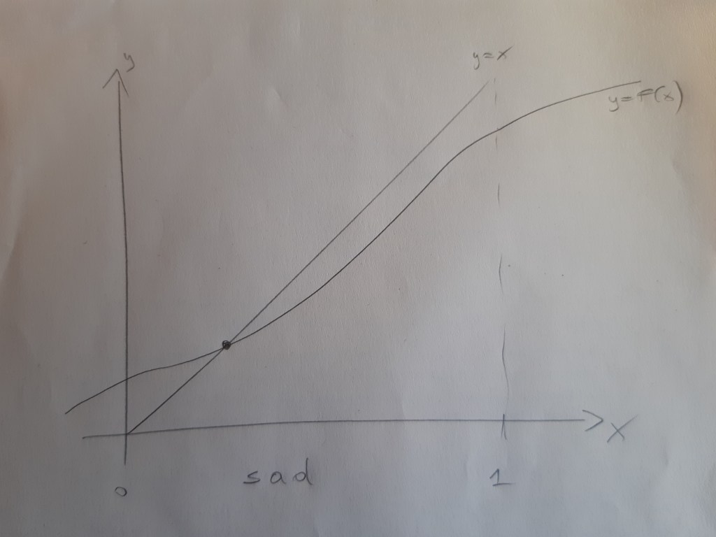
In contrast, in the picture that I titled “sad”, most people are very worried about societal shame. This can be seen in the slow rise of
in
How could we get from the latter situation to the former? There are, actually, many ways a government could try to make that happen. One option would be to make helmets mandatory (and to enforce this rule at least to some extent) so that, presumably, people suffer a cost for not wearing a helmet, the fine they might receive when caught, which makes wearing a helmet relatively more attractive for them. This could be expensive, as you need to hire and pay police personnel to enforce the rules. Another option that the government could try to use is to fund an advertising campaign aimed at making people less worried about not being cool. They could try to make wearing helmets cool, instead, for instance. This could have just the same effect. Under both policy measures, if done well, the function
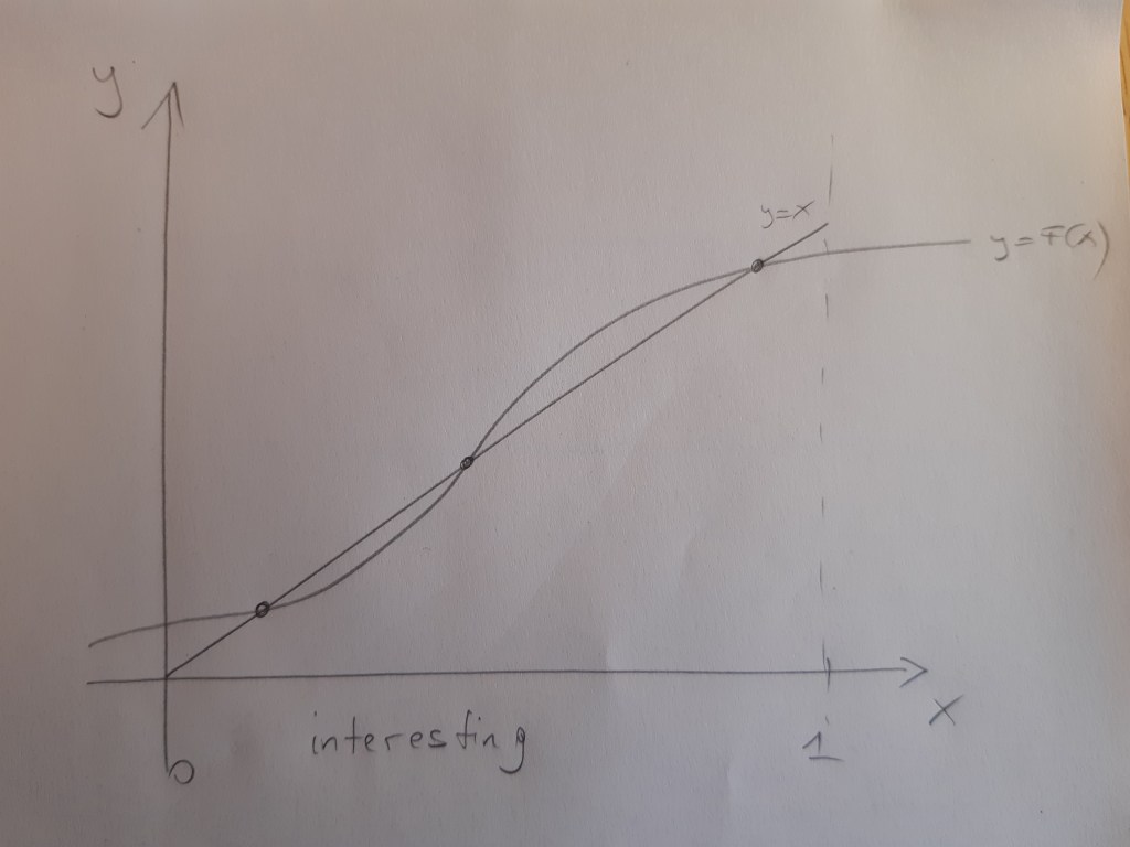
There is a third possible situation, that I depict in the figure entitled “interesting,” in which there are multiple equilibria. The low and high helmet-wearing equilibria are both dynamically stable (a dynamic process as the one I described above would lead to these points when the system starts in the vicinity of these points). The middle equilibrium is not dynamically stable. The lower equilibrium is initially more likely, as it makes sense to think that at some initial point, nobody wore helmets. If this is the situation that we are facing, then introducing a law to make helmets mandatory needs to be implemented and enforced only for a short time, until the proportion of helmet wearers exceeds the middle (unstable) equilibrium. After that we end up in the good equilibrium without any need for further enforcement.
This post has become a bit longer than I intended. Of course, one could debate whether or not there really is a social dilemma here (meaning my utility functions are possibly wrong). Perhaps, people just value the freedom of having the wind blow through their hair when scooting much more than the added chance of survival from a possible accident. Then a helmet law would make everybody just worse off. An advertising campaign might not be so bad in that case. There are many other things one could question, but I won’t do this now.


-
Subscribe
Subscribed
Already have a WordPress.com account? Log in now.
